Dynamic Programming

Dynamic programming is a technique that breaks the problems into sub-problems, and saves the result for future purposes so that we do not need to compute the result again. The subproblems are optimized to optimize the overall solution is known as optimal substructure property. The main use of dynamic programming is to solve optimization problems. Here, optimization problems mean that when we are trying to find out the minimum or the maximum solution of a problem. The dynamic programming guarantees to find the optimal solution of a problem if the solution exists.

The definition of dynamic programming says that it is a technique for solving a complex problem by first breaking into a collection of simpler subproblems, solving each subproblem just once, and then storing their solutions to avoid repetitive computations.

Let's understand this approach through an example.

Consider an example of the Fibonacci series. The following series is the Fibonacci series:

0, 1, 1, 2, 3, 5, 8, 13, 21, 34, 55, 89, 144, ,…

The numbers in the above series are not randomly calculated. Mathematically, we could write each of the terms using the below formula:

F(n) = F(n-1) + F(n-2),

With the base values F(0) = 0, and F(1) = 1. To calculate the other numbers, we follow the above relationship. For example, F(2) is the sum f(0) and f(1), which is equal to 1.

How can we calculate F(20)?

The F(20) term will be calculated using the nth formula of the Fibonacci series. The below figure shows that how F(20) is calculated.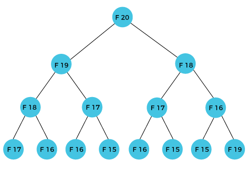

As we can observe in the above figure that F(20) is calculated as the sum of F(19) and F(18). In the dynamic programming approach, we try to divide the problem into the similar subproblems. We are following this approach in the above case where F(20) into the similar subproblems, i.e., F(19) and F(18). If we recap the definition of dynamic programming that it says the similar subproblem should not be computed more than once. Still, in the above case, the subproblem is calculated twice. In the above example, F(18) is calculated two times; similarly, F(17) is also calculated twice. However, this technique is quite useful as it solves the similar subproblems, but we need to be cautious while storing the results because we are not particular about storing the result that we have computed once, then it can lead to a wastage of resources.

In the above example, if we calculate the F(18) in the right subtree, then it leads to the tremendous usage of resources and decreases the overall performance.

The solution to the above problem is to save the computed results in an array. First, we calculate F(16) and F(17) and save their values in an array. The F(18) is calculated by summing the values of F(17) and F(16), which are already saved in an array. The computed value of F(18) is saved in an array. The value of F(19) is calculated using the sum of F(18), and F(17), and their values are already saved in an array. The computed value of F(19) is stored in an array. The value of F(20) can be calculated by adding the values of F(19) and F(18), and the values of both F(19) and F(18) are stored in an array. The final computed value of F(20) is stored in an array.

How does the dynamic programming approach work?

The following are the steps that the dynamic programming follows:

• It breaks down the complex problem into simpler subproblems.
• It finds the optimal solution to these sub-problems.
• It stores the results of subproblems (memoization). The process of storing the results of subproblems is known as memorization.
• It reuses them so that same sub-problem is calculated more than once.
• Finally, calculate the result of the complex problem.

The above five steps are the basic steps for dynamic programming. The dynamic programming is applicable that are having properties such as:

Those problems that are having overlapping subproblems and optimal substructures. Here, optimal substructure means that the solution of optimization problems can be obtained by simply combining the optimal solution of all the subproblems.

In the case of dynamic programming, the space complexity would be increased as we are storing the intermediate results, but the time complexity would be decreased.

Approaches of dynamic programming

There are two approaches to dynamic programming:

• Top-down approach
• Bottom-up approach

Top-down approach

The top-down approach follows the memorization technique, while bottom-up approach follows the tabulation method. Here memorization is equal to the sum of recursion and caching. Recursion means calling the function itself, while caching means storing the intermediate results.

Advantages

• It is very easy to understand and implement.
• It solves the subproblems only when it is required.
• It is easy to debug.

Disadvantages

It uses the recursion technique that occupies more memory in the call stack. Sometimes when the recursion is too deep, the stack overflow condition will occur.

It occupies more memory that degrades the overall performance.

Let's understand dynamic programming through an example.

In the above code, we have used the recursive approach to find out the Fibonacci series. When the value of 'n' increases, the function calls will also increase, and computations will also increase. In this case, the time complexity increases exponentially, and it becomes 2ⁿ.

One solution to this problem is to use the dynamic programming approach. Rather than generating the recursive tree again and again, we can reuse the previously calculated value. If we use the dynamic programming approach, then the time complexity would be O(n).

When we apply the dynamic programming approach in the implementation of the Fibonacci series, then the code would look like:

In the above code, we have used the memorization technique in which we store the results in an array to reuse the values. This is also known as a top-down approach in which we move from the top and break the problem into sub-problems.

Bottom-Up approach

The bottom-up approach is also one of the techniques which can be used to implement the dynamic programming. It uses the tabulation technique to implement the dynamic programming approach. It solves the same kind of problems but it removes the recursion. If we remove the recursion, there is no stack overflow issue and no overhead of the recursive functions. In this tabulation technique, we solve the problems and store the results in a matrix.

There are two ways of applying dynamic programming:

• Top-Down
• Bottom-Up

The bottom-up is the approach used to avoid the recursion, thus saving the memory space. The bottom-up is an algorithm that starts from the beginning, whereas the recursive algorithm starts from the end and works backward. In the bottom-up approach, we start from the base case to find the answer for the end. As we know, the base cases in the Fibonacci series are 0 and 1. Since the bottom approach starts from the base cases, so we will start from 0 and 1.

Key points

• We solve all the smaller sub-problems that will be needed to solve the larger sub-problems then move to the larger problems using smaller sub-problems.
• We use for loop to iterate over the sub-problems.
• The bottom-up approach is also known as the tabulation or table filling method.

Let's understand through an example.

Suppose we have an array that has 0 and 1 values at a[0] and a[1] positions, respectively shown as below: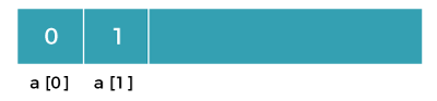

Since the bottom-up approach starts from the lower values, so the values at a[0] and a[1] are added to find the value of a[2] shown as below: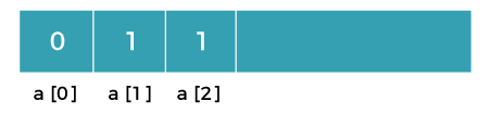

The value of a[3] will be calculated by adding a[1] and a[2], and it becomes 2 shown as below: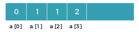

The value of a[4] will be calculated by adding a[2] and a[3], and it becomes 3 shown as below: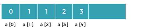

The value of a[5] will be calculated by adding the values of a[4] and a[3], and it becomes 5 shown as below: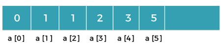

The code for implementing the Fibonacci series using the bottom-up approach is given below:

In the above code, base cases are 0 and 1 and then we have used for loop to find other values of Fibonacci series.

Let's understand through the diagrammatic representation.

Initially, the first two values, i.e., 0 and 1 can be represented as: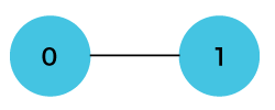

When i=2 then the values 0 and 1 are added shown as below: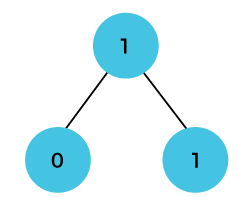

When i=3 then the values 1and 1 are added shown as below: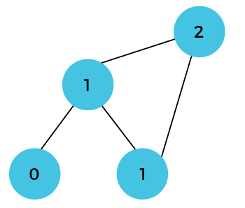

When i=4 then the values 2 and 1 are added shown as below: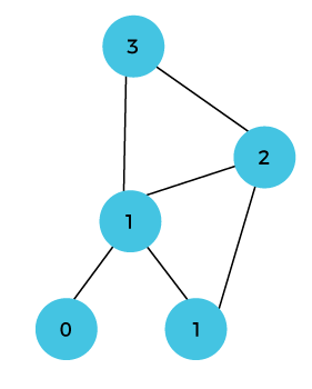

When i=5, then the values 3 and 2 are added shown as below: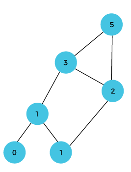

In the above case, we are starting from the bottom and reaching to the top.