Excel IF Function

MS Excel, or Microsoft Excel, is a powerful spreadsheet program that enables users to record large amounts of data in cells within multiple worksheets. Additionally, it allows users to perform various mathematical calculations and analytical operations on recorded data using a wide range of existing functions and formulas. The IF function is one such built-in widely used, most popular Excel function.

In this tutorial, we discuss the brief introduction of the Excel IF Function. The tutorial also discusses the step-by-step process of using the Excel IF function, including the relevant examples.

What is the IF Function in Excel?

The Excel IF function performs a logical comparison between two values (or cells containing values). The function evaluates if the supplied condition satisfies and then returns an output value depending on whether the result of the condition is TRUE or FALSE. In particular, the IF function is an inbuilt conditional function that returns a value based on the fulfillment or non-fulfillment of the supplied condition.

For example, we can use the IF function to compare two values, whether the value in cell A1 is greater than that in cell B1. If the conditions satisfy, it results as the TRUE; otherwise, FALSE.

The working of the Excel IF function is almost similar to the appropriately structured Flow Chart. The function is mainly useful when making logical interpretations for decision-making. We can also extend the logical test functionality of the Excel IF function by combining it with other logical functions, such as AND, OR, etc.

Syntax of IF Function

The syntax of the Excel IF function is defined as below:

Where, the 'logical_test', 'value_if_true', and 'value_if_false' are the three parts or arguments in the IF function.

Based on the above syntax, the general format of the Excel IF function is defined as below:

=IF(A1>B2, "TRUE", "FALSE")

We separated the different arguments (or parts) in the IF formula by a Comma (,). However, we can also use the Semicolon (;) based on the language settings of the machine/ device.

Arguments of IF Function

The IF Formula in Excel accepts the following three arguments:

• Logical_test: It is the first and the mandatory argument. It helps us specify the condition to be tested or evaluated as either TRUE or FALSE. The specified condition can be a value or a logical expression.
• Value_if_true: It is an optional argument accepted by the IF function. It helps us specify the value that we need to return as output when the given condition (logical_test) is 'TRUE'.
• Value_if_false: It is another optional argument accepted by the IF function. It helps us specify the value that we need to return as output when the given condition (logical_test) is 'FALSE'.

General Flow Chart Structure of Excel IF Function

As discussed above, the IF function works on the concept of a flow chart. Depending on the condition and usage of several logical functions, the flow chart of the IF function may appear to range from simple to complex accordingly. We can draw a flow chart of generic IF function like below: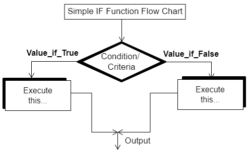

The above flow chart shows that there is only one condition or criteria, while the two outcomes are based on condition satisfaction. If the condition is satisfied (evaluated as TRUE), the function returns the value from the left box. If the condition is not satisfied (evaluated as false), the function returns the output from the other side.

Logical Operators used in IF function

The Excel IF formula typically uses logical operators to compare the values based on the given condition. When evaluating a test using the IF function, we can use any of the below logical operators:

How to use the IF Function in Excel?

To use the IF function in our Excel sheet, we must perform the following steps:

• First, we must enter or type the equal sign (=) to start the function name.
• Next, we must type the function name, followed by the starting bracket, i.e., =IF(.
• In the next step, we need to give the function the first argument (logical_test). We must specify the condition using operators' signs for logical comparison.
• After that, we need to give optional arguments, returning a value as an output based on the TRUE or FALSE.

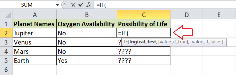
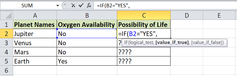
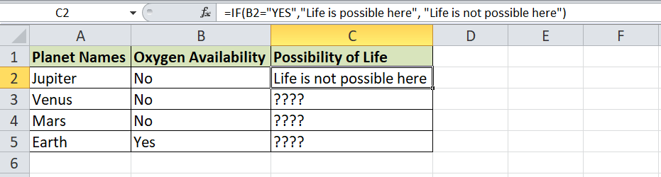
Excel IF Function Examples

Let us understand the concept and working of the Excel IF Function better with the help of the following examples:

Example 1: Basic IF Function application for empty/ non-empty cell

Everyone knows that life is not possible without oxygen. Suppose we have the following excel sheet as an example data set where column A contains the list of some planets and column B contains data about the availability of oxygen for these planets.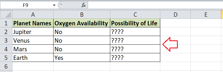

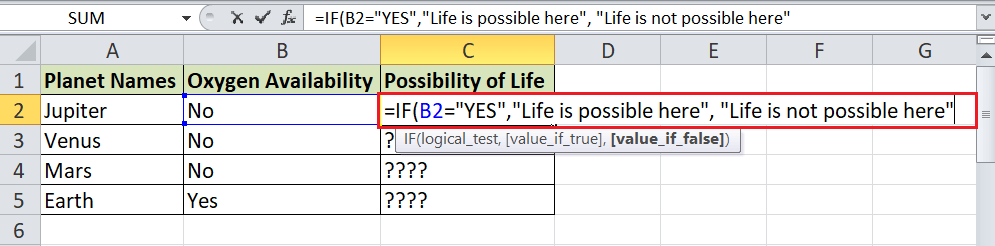
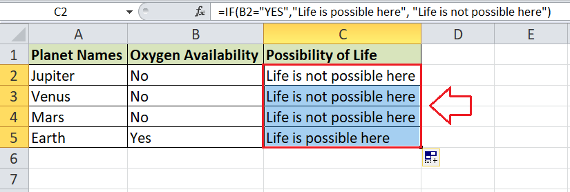
We only need to use the Excel IF function to find the planets where life is possible. We can use the oxygen availability criteria in the IF function to get the desired result. Let us now put the IF formula in our resulting column C (cells C2 to C5) and find the names of the planets with the potential for life among the planets listed in our example sheet:

• First, we find the possibility of life on the first planet (i.e., Jupiter). So, we select the respective resultant cell C2 and start the formula by entering an equal sign. After that, we enter the IF function name and the starting bracket, as shown below:
  
• Next, we apply the condition for the first planet. Since we are checking for oxygen availability as the life factor, we apply the condition (B2="YES") as B2 has data for oxygen availability. It will look like this:
  
• Lastly, we give values to be returned based on the satisfaction and dissatisfaction of the condition. If the condition matches, we want the IF function to return: 'Life is possible here'. If the condition does not match, we want the IF function to return: 'Life is not possible here'. We use the Comma (,) to separate the arguments. So, the entire formula looks like this:
  
  After that, we type the closing bracket and press the Enter key to get the corresponding result. This provides the result that life is not possible on Jupiter.
  
• After finding the result for the first planet, we can apply the IF formula in the remaining resultant cells accordingly. However, it will be easier to copy-paste the formula from C2 to other cells below. Also, we can drag the formula using the Fill Handle. This will help us perform the task quickly.
  

IF function based on equal to

The IF function based on equal to condition checks whether the given number is equal to the specified value.

Example: Check whether the specified data is equal to some value.

The steps to be followed are:

Step 1: Enter the data in the worksheet, namely A1:C7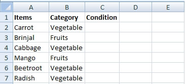

Step 2: The items and categories of fruits and vegetables are given in the data. In cell C2, enter the Formula as =IF (B2="Vegetables," "Nutrients," "Vitamins"). Suppose the data in cell range B2:B7 equal the Vegetable category. In that case, the result is displayed as Nutrients, or if the data present in the cell belongs to the Fruits Category, the result is displayed as "Vitamins."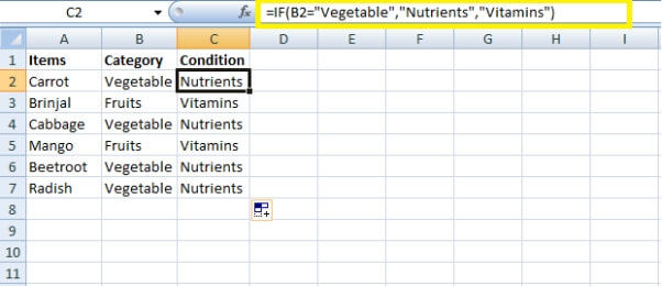

Step 3: The Fill Handle option fills the Formula for the remaining cells, which displays the required result.

IF function based on Greater than

The IF function based on the greater than condition checks whether the given number exceeds the specified value.

Example: Check whether the specified data is greater than some value.

The steps to be followed are:

Step 1: Enter the data in the worksheet, namely A1:C7

Step 2: To check whether the cost of each product is higher than 1000, enter the Formula in the cell D2 as =IF (C2>1000, "Yes," "No")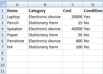

Step 3: The Fill Handle option fills the Formula for the remaining cells, which displays the required result.

IF function based on Lesser than

The IF function based on the lesser than condition checks whether the given number is lesser than the specified value.

Example: Check whether the specified data is lesser than some value.

The steps to be followed are:

Step 1: Enter the data in the worksheet, namely A1:C7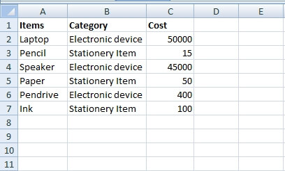

Step 2: To check whether the cost of each product is lesser than 1000, enter the Formula in the cell D2 as =IF (C2<1000, "Yes," "No")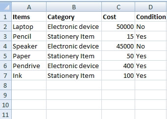

The Formula returns the result as "True" or "False" based on the conditions.

IF Function using NOT function(<>)

The IF function and the function on(<>) are used to check various criteria in the selected cell.

The steps to be followed are:

1. Enter the data in the cell range A1:A5

2. To check whether the cell range is not blank, enter the Formula in cell B1 as =IF(A1<>",1,0). Press Enter.

The Function returns the value one if the cell is not blank and returns the value zero if the 3. cell is blank.

4. Use the fill handle to display the result for the remaining cells.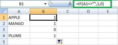

The IFS Function

The IFS function is an inbuilt function in Excel and is used to check two or more conditions for the given data.

The syntax for the IFS Function is as follows:

=IFS (logical_test1, value_if_true1, [logical_test 2, value_if_true2], [logical_test3 ;...)

The IFS function has three logical conditions:

If the given number is more significant than (>), another number

If the given number is equal to (=), another number

If the given number is lesser than (<), another number

Example: Check multiple conditions for the given data using IFS Function

The steps to be followed are:

Step 1: Enter the data in the worksheet range A1:D7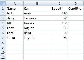

Step 2: The car driving speeds of various people are entered in the data. Multiple conditions are entered into the Formula to find the Normal, Fast, and Slow car speeds. Enter the formula in the cell D2 as =IFS (C2<50,"Slow", C2<100,"Normal", C2>100,"Fast")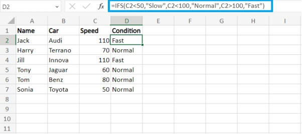

Step 3: The Fill Handle option fills the Formula for the remaining cells, which displays the required result.

Notes:

• While creating the Formula for the Nested IF function, the order in which the function is nested with each other is essential.
• Nesting multiple functions in one Formula is challenging to maintain and sometimes hard to create.
• An alternative for the Nested if Function is the VLOOLUP formula, INDEX Formula, MATCH, etc.

IF ERROR

The IF ERROR is one of the standard functions in Excel, where it handles Errors in the Formula. If the Formula contains an error, it returns an expression or a value of the expression.

The syntax of the IFERROR is:

=IFERROR (value, value_if_error)

Value- The Formula or value which needs to be evaluated for errors

Value_if_error- This value is returned if the Formula returns an error value.

The value_if_error is optional. If this option is not included in the Formula, it returns a default error message. If it is included, it displays a message about what the user has entered in the Formula.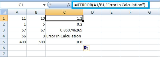

Example 2: Using IF Function with AND, OR, and MOD functions

Since the IF function can be combined with many other Excel functions, we discuss using the IF function with AND, OR, and MOD functions in this example. Suppose we have the following list of many years (1990-2022).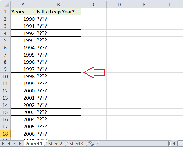

We need to determine whether a respective year is a leap year or not using the IF function. As we know that the leap year consists of 366 days, whereas February has 29 days. We find the leap year using the following concepts:

• A year exactly divisible by 4 and not exactly divisible by 100, or
• A year exactly divisible by 400

We can use any of the above two conditions and combine the IF function with AND, OR, and MOD. In the formula, the AND function typically evaluates the conditions of finding the leap years to become the respective value 'TRUE'. The OR function evaluates one of these two conditions to become the respective output as 'TRUE'. Furthermore, the MOD function will mainly help us find a remainder after a dividend is divided by a divisor.

Based on the given conditions of the leap year, we can use the MOD function in two following ways:

MOD(year,4)=0 and MOD(year,100)<>0

Or

MOD(year,400)=0

If any of the above MOD criteria are satisfied, the corresponding year is a leap year.

Now let's combine these criteria into the IF function, our formula will be:

=IF(OR(AND((MOD(year,4)=0),(MOD(year,100)<>0)),(MOD(year,400)=0)),"It is a Leap Year", "It is not a Leap Year")

Where the term 'year' is used to represent the desired year or use its corresponding cell reference from the sheet. So, when we apply the entire formula in our resultant first cell (B2), we replace the term 'year' with cell A2. It will look like this:

=IF(OR(AND((MOD(A2,4)=0),(MOD(A2,100)<>0)),(MOD(A2,400)=0)),"It is Leap Year", "It is not a Leap Year")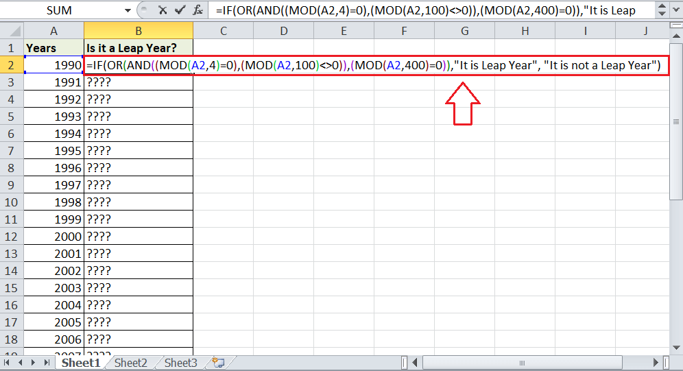

Similarly, we can apply the IF formula in other resultant cells in column B to find whether the respective years are the leap years. Once we apply the formula in all the resultant cells, our example sheet looks like this: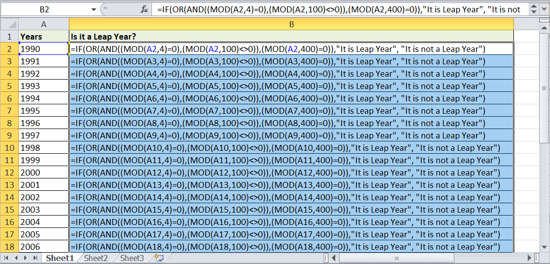

If we hide the formula in the resultant cells and check their results, we get to know which years in our list are the leap years. The following image displays that the following years 1992, 1996, 2000, 2004, 2008, 2012, 2016, and 2020 are the leap years, while others are no-leap years.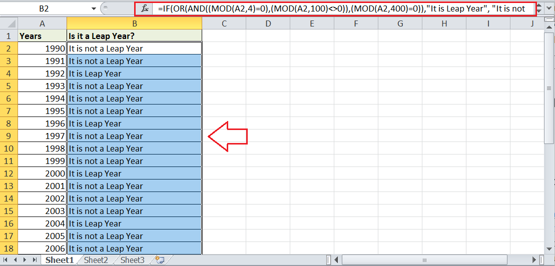

IF with NOT function

The IF function combines NOT to display the required result.

NOT Function

Example: Use the NOT Function with the IF function

1. Enter the data in the required worksheet, namely A1:B5
   
2. To check whether the data present in cell A1:A5 is NOT Pink, the value present in cell B1 is added with the result 10, or else the value in B1 is returned. Enter the formula in the cell C1 as =IF(NOT(A1="Pink"),B1+10,B1)
   
3. Use the fill handle to display the remaining cells' results.

Example 3: Using IF Function in VLOOKUP

In this example, we combine the IF function with the VLOOKUP function to make it more effective. Suppose we have the following example data sheet with a list of a few items in column A and their availability in column B.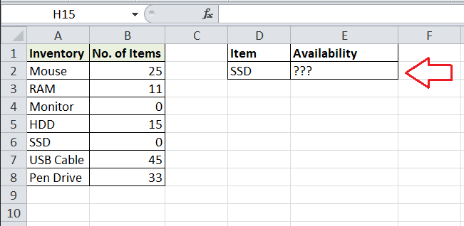

We need to use the IF function to determine whether the specific item is available in our stock (inventory). We use cell D2 to enter the item's name to be searched, while the availability of the related item will be recorded in cell E2. So, cell D2 will serve as the lookup value for the VLOOKUP function, and cell E2 will be our resulting cell to insert the entire formula.

When combining the IF function with VLOOKUP, the VLOOKUP function mainly looks up the values referring to the availability of the respective item, while the IF function checks whether the number of availability is greater than zero. If the number of items is above zero, the corresponding item is in our inventory.

Based on our example data, we can apply the VLOOKUP function in the following way:

=VLOOKUP(D2,A2:B8,2,0)

Where A2:B8 is the table array, and '2' is the column number used to return a value.

Now, we apply the condition for the item availability by combining the above VLOOKUP formula with the IF function in the following way:

=IF(VLOOKUP(D2,A2:B8,2,0)>0, "Item Available","Item Not Available")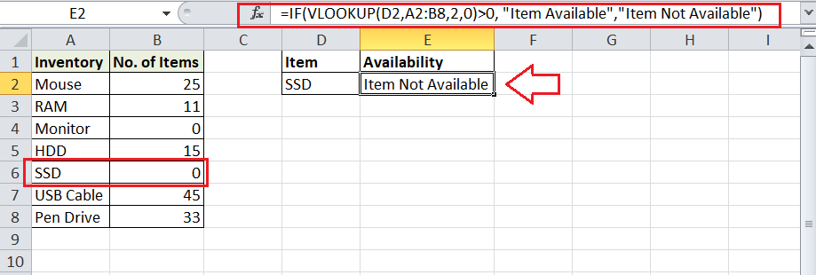

The formula returns 'Item Not Available' for the item 'SSD' in the above image. Likewise, our data table shows zero items for SSD in our inventory. So, the formula works correctly. We can change the item name in cell D2, and the item's availability will be automatically reflected in cell E2. However, the formula remains the same.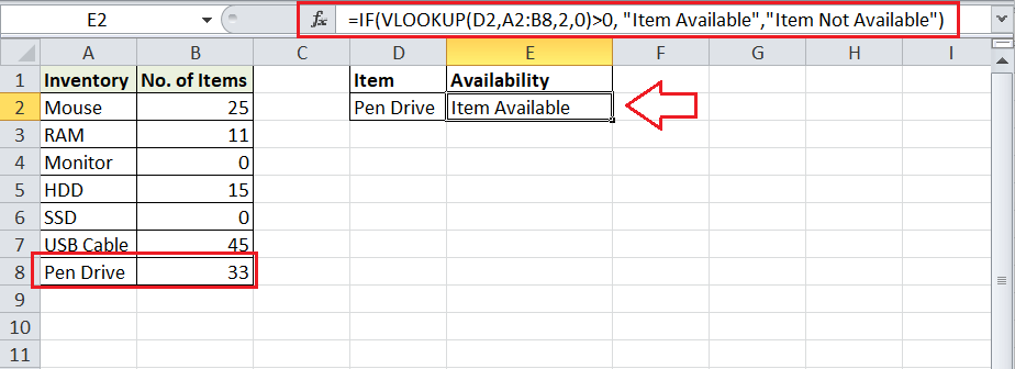

Nested IF Function

The IF function in Excel can be nested. The Nested IF Function is a combination of multiple IF functions. A 'nested IF' contains at least one IF function inside another to evaluate more than one condition at once and return the output accordingly. In Excel, up to 64 IF functions can be nested in a formula. But, we must double-check to ensure that each IF condition is correctly nested inside the other.

The following example shows the use of nested IF where IF functions are used (nested) inside another.

The condition in the IF function is used to find the corresponding grade based on the scores. The reasoning for assigning grades is in the table below:

We usually move in a nested IF formula in one direction, whether from high to low or low to high. In our example, we go from low to high. We start by testing to find grades for scores below 60, then move on to the next IF function and test grades for scores below 70, and so on. This way, we allow the function to return output (grade) only if the condition is TRUE, and the function checks the next IF condition only if the previous function has already returned FALSE.

Note: Instead of using the multiple nested IF functions, we can use an IFS function in Excel. However, the IFS function is only available in Office 2019 and Microsoft 365. In older versions, we can consider using VLOOKUP or HLOOKUP because they can handle many conditions properly, even in complex situations.

IF function with specific text

The IF function does not support wildcards. Hence the combination of ISNUMBER and SEARCH Function is used to find the specific text in the given data.

Example: Find the specific text using ISNUMBER and SEARCH Function.

Step 1: Enter the data in the worksheet, namely A1:A5

Step 2: To determine whether the particular string is present in cell A1, enter the Formula in cell B1 as =IF(ISNUMBER(SEARCH("ABC," A1)), "Yes," "No")

Step 3: If the specified data is present in the cell, the Function returns the result as Yes, or it returns the result as No.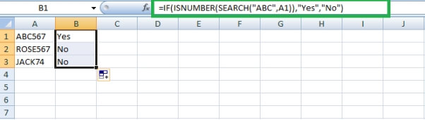

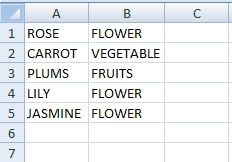
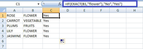
Step 4: Use the fill handle to display the remaining cells' results.

IF Function for Case-sensitive Data

To differentiate the upper case and lower case characters, the IF function, along with the EXACT function, is used.

The steps to be followed are:

1. Enter the data in the worksheet, namely A1:B5
   
2. Enter the Formula in the cell C1 as =IF(EXACT(B1, "flower"), "No," "Yes"). Press Enter. The result will be displayed in cell C1 based on case-sensitive data.
   
3. Use the fill handle to display the result for the remaining cells.

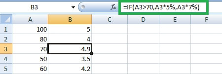
IF Formula executing another formula

The IF formula is used to execute another formula using specific criteria. The steps to be followed are:

1. Enter the data in the cell range A1:A5
2. In cell B1 enter the formula as =IF(A1>70,A1*5%,A1*7%). Press Enter. ThFunctionon multiplies the data with 5% if the value is greater than 70, or else it multiplies the data with 7%.
   
3. The fill handle displays the result for the remaining cells.

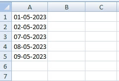
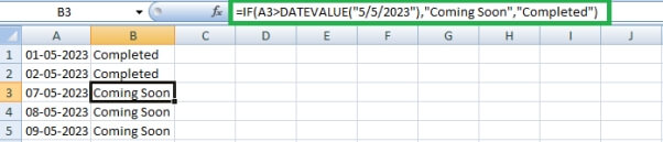
IF Function for Date

Along with text and numeric values, the IF function calculates dates. The IF function and the DATEVALUE function are used to compare the dates.

To compare the dates in the given data, the steps to be followed are :

1. Enter the dates in the required worksheet, namely A1:A5
   
2. Enter the Formula in the cell B2 as = IF(A1>DATEVALUE("5/5/2023"), "Coming Soon," "Completed")
   
3. Use the fill handle to display the remaining cells' results.

IFunctionon for Date using Absolute Reference

An alternative option to compare dates is using Absolute Reference for the specified Date.

The steps to be followed are:

1. Enter the range of data in the worksheet, A1:A5, and enter the specified Date in cell C1.

To compare the Date with the specified Date present in cell C1, enter the Formula in cell B1 as =IF(A1>$C$1, "Coming Soon," "Completed"). Press Enter, and the result will be displayed in cell B1.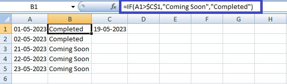

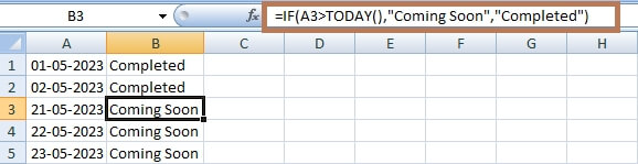
3. Use Fill Handle to display the result for the remaining cells.

IF function for Date using TODAY() Function

An alternative option to compare the dates is using the Today(Function) for the specified Date.

The steps to be followed are:

1. Enter the range of data in the worksheet, namely A1:A5.
2. To compare the Date with today's Date, enter the Formula in cell B1 as =IF(A1>TODAY(), "Coming Soon","Completed"). Press Enter, and the result will be displayed in cell B1.
   
3. Use Fill Handle to display the result for the remaining cells.

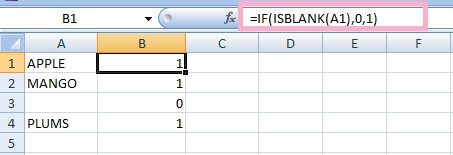
IF function using ISBLANK() Function

The ISBLANK() function with the IF function is used to check whether the cell is blank.

The steps to be followed are:

1. Enter the data in the worksheet, namely A1:A5
2. To check whether the cell range A1:A5 contains blank, enter the Formula in the cell B1 as =IF(ISBLANK(A1),0,1). The Function returns the value zero; if the cell is blank or if the cell contains data, it returns the value one
   
3. Use Fill Handle to display the result for the remaining cells.

Important Points to Remember

• The IF function does not support wildcards. However, we can use basic wildcard functionality by combining the IF function with the COUNTIF function.
• If any argument in the IF function is supplied as the array, the function evaluates each array element accordingly.
• The #NAME! error occurs for the IF formula when we type the wrong function name. For example, IFF, IEF, etc.
• The #VALUE! error for the IF formula occurs when the argument 'logical_test' is not evaluated as TRUE or FALSE.