Quick Excel Functions

Microsoft Excel, commonly called Excel, is powerful spreadsheet software that allows users to record large amounts of data sets and perform various arithmetic calculations. It is a versatile spreadsheet program for solving math problems, analyzing or comparing data, or making graphical representations of data. However, all such things in Excel are done with the help of existing functions and formulas created by us.

This tutorial discusses the list of the most used essential quick excel functions, including the relevant examples. With this tutorial, we'll learn when to use the various functions and perform basic tasks quickly without any calculators or extra work.

What is an Excel function?

An Excel function refers to a predefined formula that helps us perform a specific operation on the recorded data within the worksheet. The functions contain familiar names and eliminate the need to enter complex formulas manually. In Excel, the formulas may contain one or more functions in the equation. Since the functions are typically another form of formulas in Excel, they also start with an equal sign (=).

Basic Excel Functions that we can use quickly in Excel

Excel has over 400 predefined functions, and this number steadily increases from version to version with every upgrade. We usually don't need to memorize them all. Instead, we can access the desired function using the function wizard. However, it is beneficial to know some quick Excel functions that we often need to use. Below we discuss some basic but valuable quick Excel functions that we often need to use as a beginner:

SUM

The SUM function in Excel helps us add two or more values directly in an Excel cell. Additionally, we can also pass the cell references, ranges, or the mix of arguments. The SUM function is the most basic built-in Excel function and requires at least one argument.

The syntax of the SUM function is defined as below:

Where the number1 is the mandatory argument and may contain a number, cell reference, range, or a mix of all three. Additionally, we can add more than one argument as per our requirements.

Example: Suppose we have a list of month-wise sales data for any item, and we need to calculate the total sales for the entire year. We can use the SUM function and quickly add sales for each month. If our sales data is recorded in cells from B2 to B13, we can use the SUM function in the following way to record the yearly sales in any resultant cell:

=SUM(B2:B13)

When the above equation is entered in cell B14, we get the addition of values in the corresponding cells, as shown below: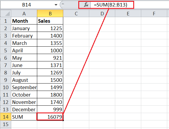

Excel also provides another quick way to record the addition of column values or rows of numbers. When we have values in an adjacent (contiguous) range, we can go to the very next cell after the data and click on the AutoSum (Shortcut: press 'Alt' and '=' keys simultaneously) button from the Home tab. This will immediately insert the SUM function and calculate the SUM of all the previous cells with numbers.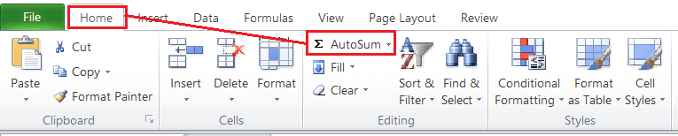

AVERAGE

The AVERAGE function in Excel is another basic function that is often used by beginners, especially when learning the concepts of Excel functions and applying them within the worksheet. As the name suggests, the function helps us calculate the average value or arithmetic mean for the given numbers.

Like other essential functions, the AVERAGE function also eliminates the need to create a formula to calculate the average manually. Instead, we only need to pass the cells or a range, and results will be calculated accordingly in the resultant cell. The function performs all the calculations behind the scenes. It first adds all the given numbers and then divides the results by the total count of given numbers.

The syntax of the AVERAGE function is defined as below:

The syntax is almost similar to the SUM function, and it is mandatory to pass at least one argument in the function. We can pass arguments as numbers, cell references, range, or a mix of all three. We can pass more than two arguments or numbers in the AVERAGE function as per our requirements.

Example: The application of the AVERAGE function is precisely similar to the SUM function. If we take the same example data of month-wise sales again, the average in cell B13 can be calculated in the following way:

=AVERAGE(B2:B13)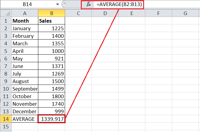

For the quick implementation of the AVERAGE function, we can select a cell next to our contiguous data set and go to Home > AutoSum drop-down (under Editing section) > Average.

COUNT

The COUNT function in Excel is another essential function used to count the total number of cells in a given range that contains numeric values. Using the COUNT function, we quickly know about the number/ count of numeric values (numbers) entries. The COUNT function usually ignores data sets other than numbers.

The syntax of the COUNT function is defined as below:

The first argument is mandatory, while we can add more arguments if required.

Example: In the previous example sheet, we have month-wise sales data. So, the total number of cells that contain numbers is 12 because we have the month from January to December. Let us now check the results using the COUNT function by giving the range in the function as follows:

=COUNT(B2:B13)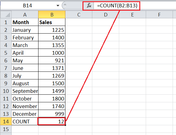

In the above image, we can see that the result is 12, the same as expected.

Suppose we enter any text value (i.e., "No Sales") in any of the cells of the range B2:B13. So, the results change to 11 because the COUNT function ignores the cells with text values.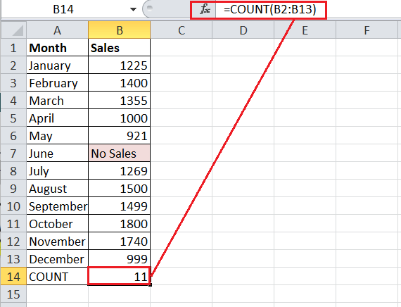

We can apply the COUNTA function to measure all the cells in a range irrespective of the numbers or text values.

For the quick implementation of the AVERAGE function, we can select a cell next to our contiguous data set and go to Home > AutoSum drop-down (under Editing section) > Count Numbers. However, it only fetches the range of the adjacent cells with numbers. So, we must double-check the range within the function.

MAX & MIN

MAX and MIN are the two different basic functions in Excel and are quick to use within the desired cell. Both functions have almost the opposite operations. The MAX function helps us get the maximum value in a given set of data, cells, or ranges. In contrast, the MIN function helps us get the minimum value in a specific range. However, the syntax and the application process of MAX and MIN functions are similar.

The syntax of the MAX function is defined as below:

The first argument is mandatory, while we can add more arguments if required.

Example: When we apply the MAX function in our month-wise sales data, we get the highest number of sales. We can use the MAX function for the range B2:B13 in the following way:

=MAX(B2:B13)

This returns 1800, the highest/ maximum number in our range.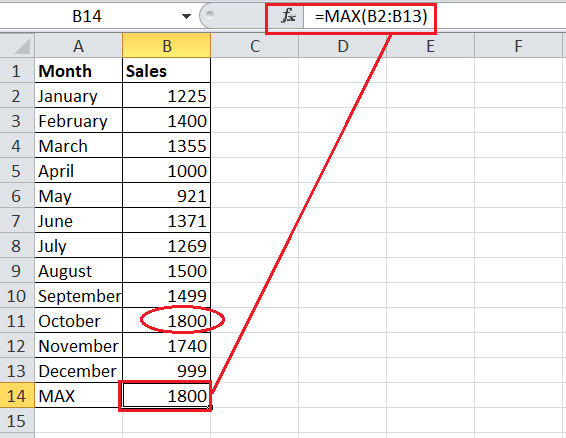

The syntax of the MIN function is defined as below:

Like the MAX function, the first argument in the MIN function is mandatory, while we can add more arguments as per our requirements.

Example: On the same example sheet, we can use the MIN function for the range B2:B13 in the following way:

=MIN(B2:B13)

This returns 921, the highest/ maximum number in our range.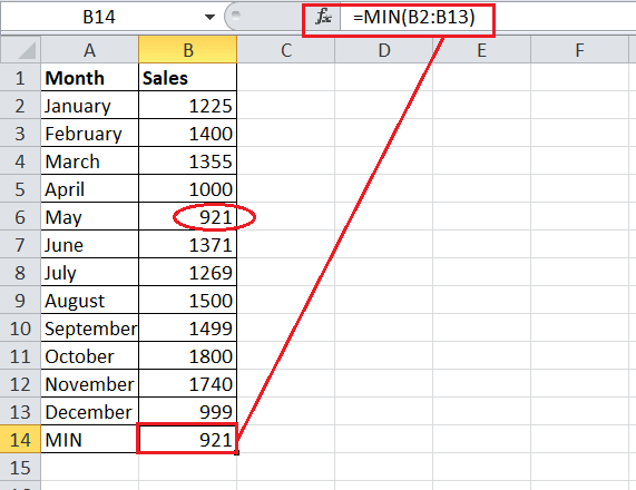

RANDBETWEEN

The RANDBETWEEN function in Excel lets us pick or record any random number from the given set of numbers, and it only returns a random integer number. The function is categorized under the Math and Trigonometry functions section. We need to specify a range of numbers by passing a minimum and maximum number in a formula.

The syntax of the RANDBETWEEN function is defined as below:

Here, we must specify the lowest number as the bottom argument and the highest number as the top argument in the formula.

Example: Suppose we have a list of 10 people, and we want to pick any random person amongst them for any specific purpose (for example- choosing a winner randomly). We can use the RANDBETWEEN function and pass respective arguments in the following way:

=RANDBETWEEN(1, 10)

This will return a random number between 1 and 10. Each time we apply it to the cell, the value returned can be the same or different.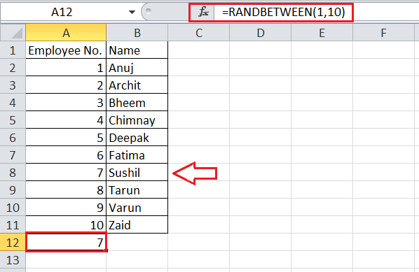

TRIM

When creating formulas in an Excel cell, we often encounter unexpected error codes instead of the expected results. The formula returns errors due to several reasons. One of the most common causes of formula errors may be the presence of unnecessary spaces in a cell. Therefore, we may need to remove such unwanted spaces in our worksheets. However, deleting the extra spaces within the large data set might be somewhat tricky if we try to check and delete them manually. This is where the TRIM function is helpful.

Although there are multiple ways to delete extra unwanted spaces from our worksheet, the TRIM function makes it more accessible. The function eliminates all extra spaces in given cells but retains a single space character between two or more words.

The syntax of the TRIM function in Excel is defined as below:

We must pass the desired cell reference where we want to remove extra spaces.

Example: Suppose we have a list of data in column A where we see extra spaces in values. We apply the TRIM function in the following way:

=TRIM(A2)

After applying the formula in the first resultant cell B2, we copy the formula in the other cells below.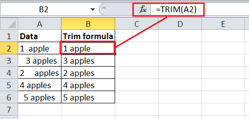

The above image shows how the TRIM function has removed the extra spaces from the data in column A and recorded the resultant values in the following column B.

LEN

The LEN function in Excel helps us know the total number of characters present in the given cell. It is essential to note that the function counts all the characters, whether numbers, text or symbols. Also, the space characters are included in the count results of the LEN function.

The syntax of the LEN function is defined as below:

We must pass the desired cell reference where we want to count the total characters.

Example: In the previous example data, we apply the LEN function in the following way:

=LEN(A2)

The formula is copied to other cells below in column B, where cell references change accordingly.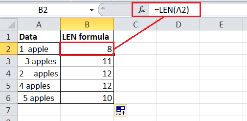

In the above image, the function calculates the total characters in values recorded in column A and records them in the subsequent column B.

CONCATENATE

The CONCATENATE function in Excel helps us quickly combine values from two or more cells into a new cell.

The syntax of the CONCATENATE function is defined as below:

Where the 'text1' is the mandatory argument; however, we can pass optional arguments if required.

Example: Suppose we want to combine values from cells A1 and B1. We can apply the CONCATENATE function in the following way:

=CONCATENATE(A1,B1)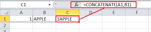

If we want to separate the combined values using the space, we can pass the space character as an argument in the CONCATENATE function in the following way:

=CONCATENATE(A1," ",B1)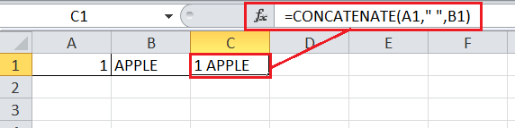

TODAY & NOW

In Excel, the TODAY and NOW are two different functions where the TODAY function helps us return the current date while the NOW function returns the current time and time both. Both functions are helpful if we don't remember the date or time but need to use them within the Excel cells. The beauty of these two functions is that we don't even need to pass any arguments in them.

We can use the syntax of TODAY and NOW functions in the following ways, respectively:

=TODAY( )

=NOW( )

Example: The following image shows how the TODAY and NOW functions are applied to record the current date and time in cells:

Quick Functions accessible from the Status Bar

Some of the functions discussed above can also be added to the status bar located at the bottom of the Excel window. Adding such functions to the status bar helps us see those functions' results without even applying them in our excel sheet. Instead, as soon as we select cells or ranges in an Excel sheet, the results of the added functions automatically appear on the status bar.

The following image shows the AVERAGE, COUNT, MINIMUM, MAXIMUM, and SUM for the selected range of cells.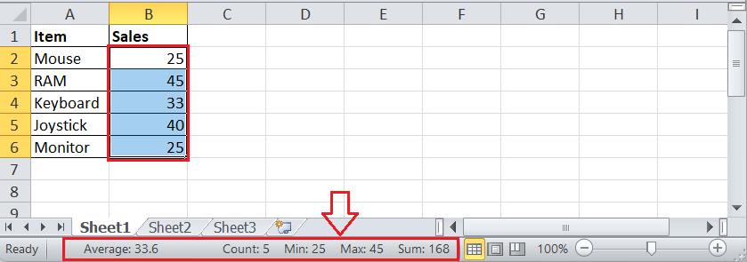

We can choose between the available functions to add to our status bar. We have to press the right-click button on the status bar and select the function to add. A tick mark/symbol appears when we select a function to add to our status bar. It looks like this: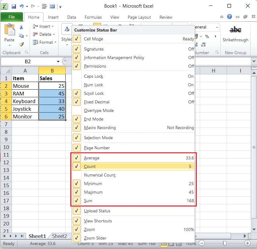

Important Points to Remember

• When using Excel functions, we must ensure not to enclose numbers within double quotes. If we use double quotation marks around the numbers, Excel will treat them as text values, which can lead to unexpected formula results.
• It is recommended never to format the numbers used in the Excel functions.
• We must ensure that each opening parenthesis has the ending parenthesis, especially when there is more than one set of parenthesis.
• Although we can copy-paste functions from one cell to another, we must ensure that the cell references are correct. It is better to use absolute references when there is a need to copy the functions/ formulas.