3D Reference in Microsoft Excel

3D references in the excel is primarily considered to be one of the greatest tool in Microsoft Excel as its cell references within the same worksheet, from one worksheet to the other, or even from one workbook to the other.

What do you mean by 3D Reference in Microsoft Excel?

"3D references are termed to be dimensional references in the analytical field. And the 3D references are then taken as a cell reference of the same cell or the same ranges from various worksheets which are termed as the 3D references in Microsoft Excel."

Besides all these, the respective 3D referenceis a new feature in Microsoft Excel, which usually allows us (or an individual) to create an efficient relationship between the various multiple worksheets in the same workbook. Moreover, this feature can also be used with the PivotTables, charts, and all other data types in Microsoft Excel.

And moving on, a simple example of this could be if we had two sheets with the sales data and wanted to view those particular sales data from both sheets simultaneously. And then, we could effectively create a 3D reference between the two sheets so that when we change one sheet, it will automatically change the other sheet very well.

Furthermore, a 3D reference combines the row and column references, allowing us to refer to the particular cell by name. For example, we will be considering the Formula that is =SUM (A1:B5). And this Formula alternatively efficiently adds out the values in cells A1 through B5. And it also makes use of the 2D reference, and this is because it only knows about respective rows as well as the columns.

How can we Set Up A 3D Reference?

We set up the 3D reference in Microsoft Excel, and then, in that particular scenario, we must select the specific cell or the range on both the sheets where we want the 3D reference set up or built build up. After once this has been done, we should go to Data > Connections > Edit Links > Create Linked Cells in Same Workbook and then after that, click on the "OK" button as this will eventually open up the dialogue box where we can specify which individual cells on each sheet would be linked together.

After that, we will look at the difference between the regular and 3D cell references in Microsoft Excel.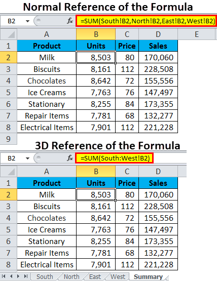

Now we will have a look at both formulas. As in the first picture (which is the Normal References), then the SUM function is applied, and the same cell reference of cell B2 of sheets South, North, East, and West will add up with the help of the SUM function.

=SUM (South! B2, North! B2, East! B2, West! B2)

Now, we will look at the 3D Formula or the reference in Microsoft Excel. And the SUM function is applied over it, but the cell reference (B2) will gets appears only once, unlike the standard connection in which the cell reference (B2) basically occurs more than 4 times.

Moreover, the particular 3D references will efficiently show how many sheets are getting involved here and then after that it will show only the first as well as the last sheet names and the same cell (B2) of those sheets efficiently.

=SUM (South: West! B2)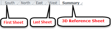

The 3D formulas or the particular reference take out the same cell of the first sheet, the last sheet, and then in-between the sheet, the same cell reference. As we have already explained that the particular Formula will only shows the first sheet, the last sheet, and the cell references.

How to make use of the 3D Reference in Microsoft Excel?

The respective 3D reference in Microsoft Excel is considered very simple and easy to handle by any user.

# Example: 1 Consolidate Excel Sheets by the help of the 3D References or Formula

As it was well known that the particular Consolidate function takes out the extra time in order to consolidate many of the sheets if the particular link sheet option is not selected out then it would not be considered as the dynamic function. But the respective 3D formulas can also be updated quickly, as it is not time-consuming.

Besides all these, we have four sheet sales values of 4 different regions, as seen in the below-attached screenshot.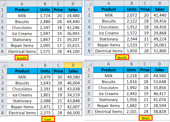

After that, if we want to consolidate all the available sheets into one sheet, that is termed the SUMMARY Sheet. And for this, we have already created the respective template, as depicted in the screenshot below.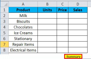

After creating a template sheet, we will follow the steps below to create 3D references or the particular formulas in Microsoft Excel.

Step 1: In the first step, we will move to the SUMMARY Sheet and then, after that, will open the SUM formula in cell B2, as it was depicted in the below-attached screenshot.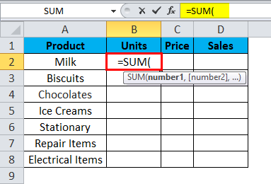

Step 2: Now, after that, we will go to the first sheet of the four different region sheets, which means the SOUTH sheet, and then select cell B2, as seen in the below-attached screenshot.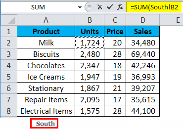

Step 3:After that, we have to do nothing but hold the SHIFT key and then directly select the last sheet in the respective workbook, which means the WEST sheet with our mouse, as it was depicted in the below-attached screenshot.

Step 4:Now, after that, we must see the Formula like this in the formula bar, as can be seen in the below-attached screenshot respectively.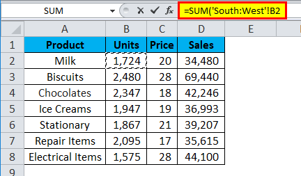

Step 5: After that, in this step, we will now "Hit" the ENTER button to complete the 3D formula reference, as these can be effectively seen in the below-attached figure respectively.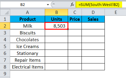

Step 6: Now, we will drag out the Formula across the summary table by pressing the shortcut keys that are CTRL+D first and then pressing Ctrl+A later. Now the result is as seen in the below depicted figure.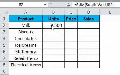

# Example: 2 Including of the New Worksheet in the 3D

It was known that the 3D reference as well as the formulas is very much flexible. As seen in the previous example, we have four sheets which in turn used to consolidate out the data in a single sheet.

Besides that, we will now, assume that we are needed to add one more of the sheet to the 3D Formula or in the reference; then the question arises: how to add to the existing 3D Formula? And if we are so confused about how to add, then follow the below mentioned steps to get overcome that obstacle:

Step 1:In the very first step, we will insert a new sheet into the workbook and then rename it accordingly, as seen in the figure below.

Step 2:Now in these step, we will now insert out the new sheet and then after that, we will placed the newly inserted sheet in between of the first as well as in the last sheet of the 3D reference sheets, that means just after the SOUTH sheet and before the WEST sheet, as it can be seen in the below-attached figure.

Step 3: Now in these step, we will see that it is much visible that there is no more amount of value in cell B2 in the newly inserted sheet efficiently. Then, in that case, we need to enter some of the importance of cell B2, as seen in the below-attached screenshot.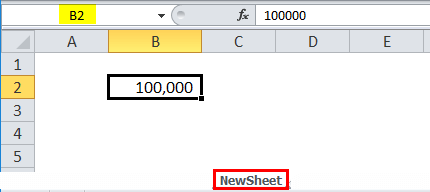

Step 4:Now after that, in this step, we will move to the SUMMARY Sheet, and then we will check out the values in cell that is cell B2. And it should also show the new deal, including the newly inserted sheet value, as depicted in the screenshot below.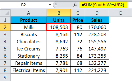

And after performing all the steps mentioned earlier in the sequences, we can easily see that the value has been changed, and we have solved the questions mentioned earlier.

Things to Remember about 3D Reference in Microsoft Excel

The various essential things as well as the points that must be remembered by an individual while working with the 3D References in Microsoft Excel, are as follows:

1. The first one is that to create the 3D reference, all the related fields across sheets must effectively be the same in Microsoft Excel.
2. Most of the specific types of functions that support the 3D formulas are none other than the following ones:
   1. MAX functions.
   2. MIN Functions.
   3. AVERAGE Functions.
   4. PRODUCT Functions.
   5. SUM functions.
   6. Etc.
3. And if the existing sheet is basically moved out of the first as well as in the last sheet, then it will eventually eliminate that respective value from the 3D Formula effectively.