Building Blocks

Neural networks are made of shorter modules or building blocks, same as atoms in matter and logic gates in electronic circuits. Once we know what the blocks are, we can combine them to solve a variety of problems.

Processing of Artificial neural network depends upon the given three building blocks:

• Network Topology
• Adjustments of weights or learning
• Activation functions

In this tutorial, we will discuss these three building blocks of ANN in detail.

Network Topology:

The topology of a neural network refers to the way how Neurons are associated, and it is a significant factor in network functioning and learning. A common topology in unsupervised learning is a direct mapping of inputs to a group of units that represents categories, for example, self-organizing maps. The most widely recognized topology in supervised learning is completely associated, three-layer, feedforward network (Backpropagation, Radial Basis Function Networks). All input values are associated with all neurons in the hidden layer (hidden because they are not noticeable in the input or the output), the output of the hidden neurons are associated to all neurons in the output layer, and the activation functions of the output neurons establish the output of the entire network. Such networks are well-known partly because hypothetically, they are known to be universal function approximators, for example, a sigmoid or Gaussian.

Feedforward network:

The advancement of layered feed-forward networks initiated in the late 1950s, given by Rosenblatt's perceptron and Widrow's Adaptive linear Element (ADLINE).The perceptron and ADLINE can be defined as a single layer networks and are usually referred to as single-layer perceptron's. Single-layer perceptron's can only solve linearly separable problems. The limitations of the single-layer network have prompted the advancement of multi-layer feed-forward networks with at least one hidden layer, called multi-layer perceptron (MLP) networks. MLP networks overcome various limitations of single-layer perceptron's and can be prepared to utilize the backpropagation algorithm. The backpropagation method was invented autonomously several times.

In 1974, Werbos created a backpropagation training algorithm. However, Werbos work remained unknown in the scientific community, and in 1985, parker rediscovers the technique. Soon after Parker published his discoveries, Rumelhart, Hinton, and Williams also rediscovered the method. It is the endeavors of Rumelhart and the other individual if the Parallel Distributed Processing (PDP) group, that makes the backpropagation method a pillar of neurocomputing.

Single-layer feedforward network:

Rosenblatt first constructed the single-layer feedforward network in the late 1950s and early 1990s. The concept of feedforward artificial neural network having just one weighted layer. In other words, we can say that the input layer is completely associated with the outer layer.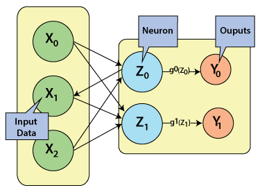

Multilayer feedforward network:

A multilayer feedforward neural network is a linkage of perceptrons in which information and calculations flow are uni-directional, from the input data to the outputs. The total number of layers in a neural network is the same as the total number of layers of perceptrons. The easiest neural network is one with a single input layer and an output layer of perceptrons. The concept of feedforward artificial neural network having more than one weighted layer. As the system has at least one layer between the input and the output layer, it is called the hidden layer.

Feedback network:

A feedback based prediction refers to an approximation of an outcome in an iterative way where each iteration's operation depends on the present outcome. Feedback is a common way of making predictions in different fields, ranging from control hypothesis to psychology. Using feedback associations is also additionally exercised by biological organisms, and the brain is proposing a vital role for it in complex cognition.

In other words, we can say that a feedback network has feedback paths, which implies the signal can flow in both directions using loops. It makes a non-linear dynamic system, which changes continuously until it reaches the equilibrium state. It may be divided into the following types:

Recurrent network:

The human brain is a recurrent neural network that refers to a network of neurons with feedback connections. It can learn numerous behaviors, sequence, processing tasks algorithms, and programs that are not learnable by conventional learning techniques. It explains the rapidly growing interest in artificial recurrent networks for technical applications. For example, general computers that can learn algorithms to map input arrangements to output arrangements, with or without an instructor. They are computationally more dominant and biologically more conceivable than other adaptive methodologies. For example, Hidden Markov models (no continuous internal states), feedforward networks, and supportive vector machines (no internal states).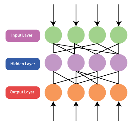

Fully recurrent network:

The most straightforward form of a fully recurrent neural network is a Multi-Layer Perceptron (MLP) with the previous set of hidden unit activations, feeding back along with the inputs. In other words, it is the easiest neural network design because all nodes are associated with all other nodes with every single node work as both input and output.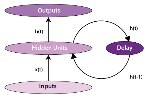

Note that the time 't' has to be discretized, with the activations updated at each time interval. The time scale may compare to the activity of real neurons, or for artificial systems whenever step size fitting for the given problem can be used. A delay unit should be introduced to hold activations until they are prepared at the next time interval.

Jordan network:

The Jordan network refers to a simple neural structure in which only one value of the process input signal (from the previous sampling) and only one value of the delayed output signal of the model (from the previous sampling) are utilized as the inputs of the network. In order to get a computationally basic MPC (Model Predictive Control) algorithm, the nonlinear Jordan neural model is repeatedly linearized on line around an operating point, which prompts a quadratic optimization issue. Adequacy of the described MPC algorithm is compared with that of the nonlinear MPC scheme with on-line nonlinear optimization performed at each sampling instant.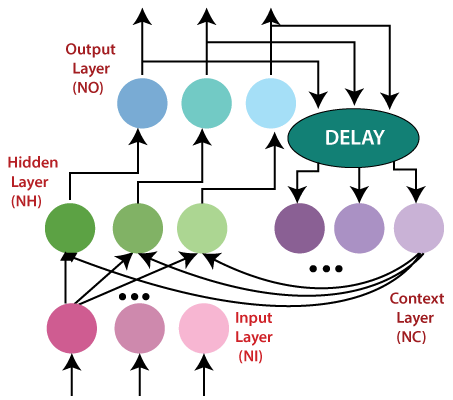

Adjustments of Weights or Learning:

Learning in ANN is the technique for changing the weights of associations between the neurons of a specified network. Learning in artificial neural networks can be characterized into three different categories, namely supervised learning, unsupervised learning, and reinforcement learning.

Supervised learning:

Supervised learning consists of two words supervised and learning. Supervise intends to guide. We have supervisors whose duty is to guide and show the way. We can see a similar case in the case of learning. Here the machine or program is learning with the help of the existing data set. We have a data set, and we assume the results of new data relying upon the behavior of the existing data sets. It implies the existing data sets acts as a supervisor or boss to find the new data. A basic example being electronic gadgets price prediction. The price of electronic gadgets is predicted depending on what is observed with the prices of other digital gadgets.

During the training of artificial neural networks under supervised learning, the input vector is given to the network, which offers an output vector. Afterward, the output vector is compared with the desired output vector. An error signal is produced if there is a difference between the actual output and the desired output vector. Based on this error signal, the weight is adjusted until the actual output is matched with the desired output.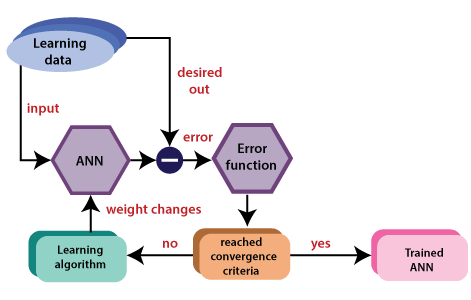

Unsupervised learning:

As the name suggests, unsupervised learning refers to predict something without any supervision or help from existing data. In this learning, the program learns by dividing the data with similar characteristics into similar groups. In supervised learning, the data are grouped, relying upon similar characteristics. In this situation, there are no existing data to look for direction. In other words, there is no supervisor. During the training of the artificial neural network under unsupervised learning, the input vectors of a comparative type are joined to form clusters. At the point when a new input pattern is implemented, then the neural network gives an output response showing the class to which the input pattern belongs. There is no feedback from the environment about what should be the ideal output and if it is either correct or incorrect. Consequently, in this type of learning, the network itself must find the patterns and features from the input data and the connection for the input data over the output.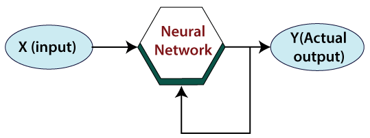

Reinforcement learning:

Reinforcement Learning (RL) is a technique that helps to solve control optimization issues. By using control optimization, we can recognize the best action in each state visited by the system in order to optimize some objective function. Typically, reinforcement learning comes into existence when the system has a huge number of states and has a complex stochastic structure, which is not responsible to closed-form analysis. If issues have a relatively small number of states, then the random structure is relatively simple, so that one can utilize dynamic programming.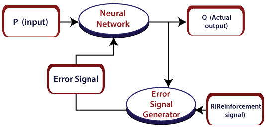

As the name suggests, this kind of learning is used to strengthen the network over some analyst data. This learning procedure is like supervised learning. However, we may have very little information. In reinforcement learning, during the training of the network, the network gets some feedback from the system. This makes it fairly like supervised learning. The feedback acquired here is evaluative, not instructive, which implies there is no instructor as in supervised learning. After getting the feedback, the networks perform modifications of the weights to get better Analyst data in the future.

Activation Function:

Activation functions refer to the functions used in neural networks to compute the weighted sum of input and biases, which is used to choose the neuron that can be fire or not. It controls the presented information through some gradient processing, normally gradient descent. It produces an output for the neural network that includes the parameters in the data.

Activation function can either be linear or non-linear, relying on the function it shows. It is used to control the output of outer neural networks across various areas, such as speech recognition, segmentation, fingerprint detection, cancer detection system, etc.

In the artificial neural network, we can use activation functions over the input to get the precise output. These are some activation functions that are used in ANN.

Linear Activation Function:

The equation of the linear activation function is the same as the equation of a straight line i.e.

Y= MX+ C

If we have many layers and all the layers are linear in nature, then the final activation function of the last layer is the same as the linear function of the first layer. The range of a linear function is –infinitive to + infinitive.

Linear activation function can be used at only one place that is the output layer.

Sigmoid function:

Sigmoid function refers to a function that is projected as S - shaped graph.

A = 1/(1+e^-x)

This function is non-linear, and the values of x lie between -2 to +2. So that the value of X is directly proportional to the values of Y. It means a slight change in the value of x would also bring about changes in the value of y.

Tanh Function:

F(x)= tanh(x) = 2/(1+e^-2X) - 1

OR

Tanh (x) = 2 * sigmoid(2x) - 1