Hopfield Network

Hopfield network is a special kind of neural network whose response is different from other neural networks. It is calculated by converging iterative process. It has just one layer of neurons relating to the size of the input and output, which must be the same. When such a network recognizes, for example, digits, we present a list of correctly rendered digits to the network. Subsequently, the network can transform a noise input to the relating perfect output.

In 1982, John Hopfield introduced an artificial neural network to collect and retrieve memory like the human brain. Here, a neuron is either on or off the situation. The state of a neuron(on +1 or off 0) will be restored, relying on the input it receives from the other neuron. A Hopfield network is at first prepared to store various patterns or memories. Afterward, it is ready to recognize any of the learned patterns by uncovering partial or even some corrupted data about that pattern, i.e., it eventually settles down and restores the closest pattern. Thus, similar to the human brain, the Hopfield model has stability in pattern recognition.

A Hopfield network is a single-layered and recurrent network in which the neurons are entirely connected, i.e., each neuron is associated with other neurons. If there are two neurons i and j, then there is a connectivity weight w_ij lies between them which is symmetric w_ij = w_ji.

With zero self-connectivity, W_ii =0 is given below. Here, the given three neurons having values i = 1, 2, 3 with values X_i=±1 have connectivity weight W_ij.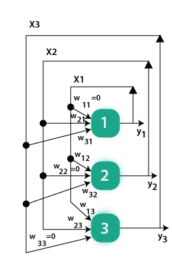

Updating rule:

Consider N neurons = 1, … , N with values X_{i =}+1, -1.

The update rule is applied to the node i is given by:

If h_i _{≥ 0} then x_i _→ 1 otherwise x_{i →} -1

Where h_i= is called field at i, with b£ R a bias.

Thus, x_i _→ sgn(h_i), where the value of sgn(r)=1, if r ≥ 0, and the value of sgn(r)=-1, if r < 0.

We need to put b_i=0 so that it makes no difference in training the network with random patterns.

We, therefore, consider h_i=.

We have two different approaches to update the nodes:

Synchronously:

In this approach, the update of all the nodes taking place simultaneously at each time.

Asynchronously:

In this approach, at each point of time, update one node chosen randomly or according to some rule. Asynchronous updating is more biologically realistic.

Hopfield Network as a Dynamical system:

Consider, K = {-1, 1} ^N so that each state x £ X is given by x_i£ { -1,1 } for 1 ≤ I ≤ N

Here, we get 2^N possible states or configurations of the network.

We can describe a metric on X by using the Hamming distance between any two states:

P(x, y) = # {i: xi≠y_i}

N Here, P is a metric with 0≤H(x,y)≤ N. It is clearly symmetric and reflexive.

With any of the asynchronous or synchronous updating rules, we get a discrete-time dynamical system.

The updating rule up: X → X describes a map.

And Up: X → X is trivially continuous.

Example:

Suppose we have only two neurons: N = 2

There are two non-trivial choices for connectivities:

w₁₂= w₂₁= 1

w₁₂= w₂₁= -1

Asynchronous updating:

In the first case, there are two attracting fixed points termed as [-1,-1] and [-1,-1]. All orbit converges to one of these. For a second, the fixed points are [-1,1] and [1,-1], and all orbits are joined through one of these. For any fixed point, swapping all the signs gives another fixed point.

Synchronous updating:

In the first and second cases, although there are fixed points, none can be attracted to nearby points, i.e., they are not attracting fixed points. Some orbits oscillate forever.

Energy function evaluation:

Hopfield networks have an energy function that diminishes or is unchanged with asynchronous updating.

For a given state X ∈ {−1, 1} N of the network and for any set of association weights W_ij with W_ij = w_ji and w_ii =0 let,

Here, we need to update X_m to X'_m and denote the new energy by E' and show that.

E'-E = (X_m-X'_m ) ∑_i≠mWmiXi.

Using the above equation, if X_m = X_m' then we have E' = E

If X_m = -1 and X_m' = 1 , then X_m - X_m' = 2 and hm= ∑_iWmiXi ? 0

Thus, E' - E ≤ 0

Similarly if X_m =1 and X_m'= -1 then X_m - X_m' = 2 and h_m= ∑_iWmiXi < 0

Thus, E - E' < 0.

Note:
If Xm flips, then E' - E = 2Xmhm

Neurons pull in or push away from each other:

Suppose the connection weight W_ij= W_ji between two neurons I and j.

If W_ij> 0, the updating rule implies:

If X_j= 1, then the contribution of j in the weighted sum, i.e., W_ijX_j, is positive. Thus the value of X_i is pulled by j towards its value X_j= 1
If X_j= -1 then W_ijX_j, is negative, and X_i is again pulled by j towards its value X_j= -1

Thus, if W_ij> 0 , then the value of i is pulled by the value of j. By symmetry, the value of j is also pulled by the value of i.

If W_ij< 0, then the value of i is pushed away by the value of j.

It follows that for a particular set of values X_i ∈ { -1 , 1 } for;

1 ≤ i ≤ N, the selection of weights taken as W_ij= X_iX_j for;

1 ≤ i ≤ N correlates to the Hebbian rule.

Training the network: One pattern (K_i=0)

Suppose the vector x^→ = (x₁,…,x_i,…,x_N) ∈ {-1,1}^N is a pattern that we like to store in the Hopfield network.

To build a Hopfield network that recognizes x^→, we need to select connection weight W_ijaccordingly.

If we select W_ij=ɳ X_iX_j for 1 ≤ i , j ≤ N (Here, i≠j), where ɳ > 0 is the learning rate, then the value of X_iwill not change under updating condition as we illustrate below.

We have