| |

Kohonen Self- Organizing Feature MapKohonen Self-Organizing feature map (SOM) refers to a neural network, which is trained using competitive learning. Basic competitive learning implies that the competition process takes place before the cycle of learning. The competition process suggests that some criteria select a winning processing element. After the winning processing element is selected, its weight vector is adjusted according to the used learning law (Hecht Nielsen 1990). The self-organizing map makes topologically ordered mappings between input data and processing elements of the map. Topological ordered implies that if two inputs are of similar characteristics, the most active processing elements answering to inputs that are located closed to each other on the map. The weight vectors of the processing elements are organized in ascending to descending order. Wi < Wi+1 for all values of i or Wi+1 for all values of i (this definition is valid for one-dimensional self-organizing map only). The self-organizing map is typically represented as a two-dimensional sheet of processing elements described in the figure given below. Each processing element has its own weight vector, and learning of SOM (self-organizing map) depends on the adaptation of these vectors. The processing elements of the network are made competitive in a self-organizing process, and specific criteria pick the winning processing element whose weights are updated. Generally, these criteria are used to limit the Euclidean distance between the input vector and the weight vector. SOM (self-organizing map) varies from basic competitive learning so that instead of adjusting only the weight vector of the winning processing element also weight vectors of neighboring processing elements are adjusted. First, the size of the neighborhood is largely making the rough ordering of SOM and size is diminished as time goes on. At last, only a winning processing element is adjusted, making the fine-tuning of SOM possible. The use of neighborhood makes topologically ordering procedure possible, and together with competitive learning makes process non-linear. It is discovered by Finnish professor and researcher Dr. Teuvo Kohonen in 1982. The self-organizing map refers to an unsupervised learning model proposed for applications in which maintaining a topology between input and output spaces. The notable attribute of this algorithm is that the input vectors that are close and similar in high dimensional space are also mapped to close by nodes in the 2D space. It is fundamentally a method for dimensionality reduction, as it maps high-dimension inputs to a low dimensional discretized representation and preserves the basic structure of its input space. 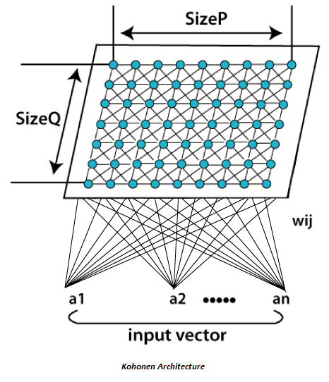
All the entire learning process occurs without supervision because the nodes are self-organizing. They are also known as feature maps, as they are basically retraining the features of the input data, and simply grouping themselves as indicated by the similarity between each other. It has practical value for visualizing complex or huge quantities of high dimensional data and showing the relationship between them into a low, usually two-dimensional field to check whether the given unlabeled data have any structure to it. A self-Organizing Map (SOM) varies from typical artificial neural networks (ANNs) both in its architecture and algorithmic properties. Its structure consists of a single layer linear 2D grid of neurons, rather than a series of layers. All the nodes on this lattice are associated directly to the input vector, but not to each other. It means the nodes don't know the values of their neighbors, and only update the weight of their associations as a function of the given input. The grid itself is the map that coordinates itself at each iteration as a function of the input data. As such, after clustering, each node has its own coordinate (i.j), which enables one to calculate Euclidean distance between two nodes by means of the Pythagoras theorem. A Self-Organizing Map utilizes competitive learning instead of error-correction learning, to modify its weights. It implies that only an individual node is activated at each cycle in which the features of an occurrence of the input vector are introduced to the neural network, as all nodes compete for the privilege to respond to the input. The selected node- the Best Matching Unit (BMU) is selected according to the similarity between the current input values and all the other nodes in the network. The node with the fractional Euclidean difference between the input vector, all nodes, and its neighboring nodes is selected and within a specific radius, to have their position slightly adjusted to coordinate the input vector. By experiencing all the nodes present on the grid, the whole grid eventually matches the entire input dataset with connected nodes gathered towards one area, and dissimilar ones are isolated. 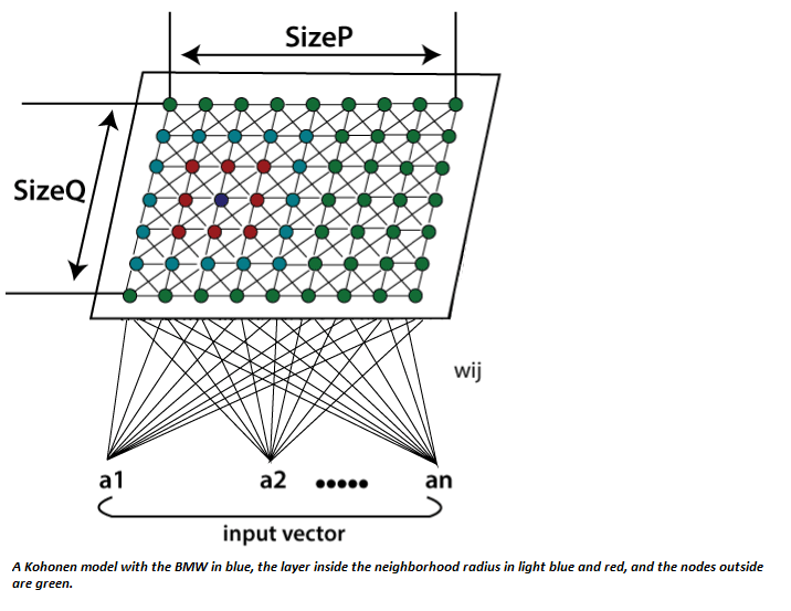
Algorithm:Step:1 Each node weight w_ij initialize to a random value. Step:2 Choose a random input vector x_k. Step:3 Repeat steps 4 and 5 for all nodes on the map. Step:4 Calculate the Euclidean distance between weight vector wij and the input vector x(t) connected with the first node, where t, i, j =0. Step:5 Track the node that generates the smallest distance t. Step:6 Calculate the overall Best Matching Unit (BMU). It means the node with the smallest distance from all calculated ones. Step:7 Discover topological neighborhood βij(t) its radius σ(t) of BMU in Kohonen Map. Step:8 Repeat for all nodes in the BMU neighborhood: Update the weight vector w_ij of the first node in the neighborhood of the BMU by including a fraction of the difference between the input vector x(t) and the weight w(t) of the neuron. Step:9 Repeat the complete iteration until reaching the selected iteration limit t=n. Here, step 1 represents initialization phase, while step 2 to 9 represents the training phase. Where; t = current iteration. i = row coordinate of the nodes grid. J = column coordinate of the nodes grid. W= weight vector w_ij = association weight between the nodes i,j in the grid. X = input vector X(t)= the input vector instance at iteration t β_ij = the neighborhood function, decreasing and representing node i,j distance from the BMU. σ(t) = The radius of the neighborhood function, which calculates how far neighbor nodes are examined in the 2D grid when updating vectors. It gradually decreases over time.
Next TopicUnsupervised Artificial Neural Networks
|
 For Videos Join Our Youtube Channel: Join Now
Feedback
- Send your Feedback to [email protected]
Help Others, Please Share


