| |

Learning and AdaptionArtificial Neural Network (ANN) is entirely inspired by the way the biological nervous system work. For Example, the human brain works. The most powerful attribute of the human brain is to adapt, and ANN acquires similar characteristics. We should understand that how exactly our brain does? It is still very primitive, although we have a fundamental understanding of the procedure. It is accepted that during the learning procedure, the brain's neural structure is altered, increasing or decreasing the capacity of its synaptic connections relying on their activity. This is the reason why more relevant information is simpler to review than information that has not been reviewed for a long time. More significant information will have powerful synaptic connections, and less applicable information will gradually have its synaptic connections weaken, making it harder to review. ANN can model this learning process by changing the weighted associations found between neurons in the network. It effectively mimics the strengthening and weakening of the synaptic associations found in our brains. The strengthening and weakening of the associations are what empowers the network to adapt. Face recognition would be an example of an issue extremely difficult for a human to precisely convert into code. An issue that could not be resolved better by a learning algorithm would be a loan granting institution that could use the previous credit score to classify future loan probabilities. The learning rule is a technique or a mathematical logic which encourages a neural network to gain from the existing condition and uplift its performance. It is an iterative procedure. In this tutorial, we will talk about the learning rules in Neural Network. Here, we will discuss what is Hebbian learning rule, perception learning rule, Delta learning rule, correlation learning rule, out star learning rule? All these Neural Network Learning Rules are discussed in details given below with their mathematical formulas. A learning rule or Learning process is a technique or a mathematical logic. It boosts the Artificial Neural Network's performance and implements this rule over the network. Thus learning rules refreshes the weights and bias levels of a network when a network mimics in a particular data environment. 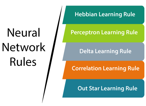
Hebbian learning rule:The Hebbian rule was the primary learning rule. In 1949, Donald Hebb created this learning algorithm of the unsupervised neural network. We can use this rule to recognize how to improve the weights of nodes of a network. The Hebb learning rule accepts that if the neighboring neurons are activated and deactivated simultaneously, then the weight associated with these neurons should increase. For neurons working on the contrary stage, the weight between them should diminish. If there is no input signal relationship, the weight should not change. If inputs of both the nodes are either positive or negative, then a positive weight exists between the nodes. If the input of a node is either positive or negative for others, a solid negative weight exists between the nodes. In the beginning, the values of all weights are set to zero. This learning rule can be utilized for both easy and hard activation functions. Since desired reactions of neurons are not utilized in the learning process, this is the unsupervised learning rule. The absolute values of the weights are directly proportional to the learning time, which is undesired. According to the Hebbian learning rule, the formula to increase the weight of connection at each time frame is given below. ∆ωij(t) = αpi(t)*qj(t) Here, ∆ωij(t) = increment by which the connection of the weight increases at the time function t. α = constant and positive learning rate. pi(t) = input value from pre-synaptic neuron at function of time t. qj(t) = output of pre-synaptic neurons at the same function of time t. We know that each association in a neural network has an associated weight, which changes throughout the learning. It is an example of supervised learning, and the network begins its learning by assigning a random variable to each weight. Here we can evaluate the output value on the basis of a set of records for which we can know the predicted output value. Rosenblatt introduces this rule. This learning rule is an example of supervised training in which the learning rule is given with the set of examples of proper network behavior: {X1,t1} , {x2,t2},…,{xq,tq} Where, Xq = input to the network. tq = target output. As each input is given to the network, the network output is compared with the objective of the network. Afterward, the learning rule changes the weights and biases the network in order to move the network output closer to the objective. Single-Neuron Perceptron: In different computer applications such as classification, pattern recognition, and prediction, a learning module can be executed by different approaches, including structural, statistical, and neural approaches. Among these techniques, artificial neural networks are inspired by the physiological operations of the brain. They depend on the scientific model of a single neural cell (neuron) named single neuron perceptron and try to resemble the actual networks of neurons in the brain. Consider a two-input perceptron with one neuron, shown in the figure given below. 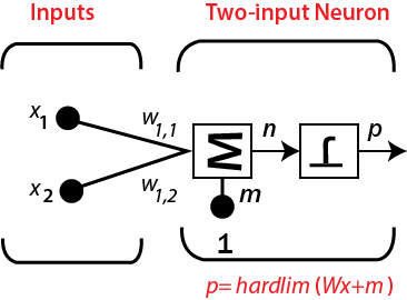
The output of this network is determined by P = hardlim(n) = hardlim(Wx + m) = hardlim( 1wTx + m) = hardlim(w1,1x1 + W1,2x2 + m) Multiple -Neuron Perceptron: For perceptron's with multiple neurons, there will be one decision boundary for individual neurons. The decision boundary of the neuron will be defined by i wT x + mi = 0 A single- neuron perceptron can classify input vectors into two classes since its output can be either null or 1. A multiple neuron perceptron can classify inputs in many classes. A different output vector shows each class. Since each component of the output vector can be either null or 1, there are a total of possible 2S possible classes, where s is the number of neurons. Mathematical equation: To describe its mathematical equation, assume we have n number of finite input vectors x n, along with its desired output vector t n, where n= 1 to N. The output 'k' can be determined, as explained earlier based on the net input, and activation function being applied over that net input can be expressed as follows: K = f (Kin)= 1, kin > θ 0, kin ≤ θ Where θ = threshold value. The various weights can be determined with respect to these two cases. Case 1 - When t ≠ k, then w(new) = w(old) + tx Case 2 – When t = k, then No change in weight Delta learning rule:The delta rule in an artificial neural network is a specific kind of backpropagation that assists in refining the machine learning/artificial intelligence network, making associations among input and outputs with different layers of artificial neurons. The Delta rule is also called the Delta learning rule. Generally, backpropagation has to do with recalculating input weights for artificial neurons utilizing a gradient technique. Delta learning does this by using the difference between a target activation and an obtained activation. By using a linear activation function, network connections are balanced. Another approach to explain the Delta rule is that it uses an error function to perform gradient descent learning. Delta rule refers to the comparison of actual output with a target output, the technology tries to discover the match, and the program makes changes. The actual execution of the Delta rule will fluctuate as per the network and its composition. Still, by applying a linear activation function, the delta rule can be useful in refining a few sorts of neural networks with specific kinds of backpropagation. Delta rule is introduced by Widrow and Hoff, which is the most significant learning rule that depends on supervised learning. This rule states that the change in the weight of a node is equivalent to the product of error and the input. Mathematical equation:The given equation gives the mathematical equation for delta learning rule: ∆w = µ.x.z ∆w = µ(t-y)x Here, ∆w = weight change. µ = the constant and positive learning rate. X = the input value from pre-synaptic neuron. z= (t-y) is the difference between the desired input t and the actual output y. The above mentioned mathematical rule cab be used only for a single output unit. The different weights can be determined with respect to these two cases. Case 1 - When t ≠ k, then w(new) = w(old) + ∆w Case 2 - When t = k, then No change in weight For a given input vector, we need to compare the output vector, and the final output vector would be the correct answer. If the difference is zero, then no learning takes place, so we need to adjust the weight to reduce the difference. If the set of input patterns is taken from an independent set, then it uses learn arbitrary connections using the delta learning rule. It has examined for networks with linear activation function with no hidden units. The error squared versus the weight graph is a paraboloid shape in n-space. The proportionality constant is negative, so the graph of such a function is concave upward with the least value. The vertex of the paraboloid represents the point where it decreases the error. The weight vector is comparing this point with the ideal weight vector. We can utilize the delta learning rule with both single output units and numerous output units. When we are applying the delta learning rule is to diminish the difference between the actual and probable output, we find an error. Correlation Learning Rule:The correlation learning rule is based on the same principle as the Hebbian learning rule. It considers that weight between corresponding neurons should be positive, and weights between neurons with inverse reactions should be progressively negative. Opposite to the Hebbian rule, the correlation rule is supervised learning. Instead of an actual response, oj (desired response), dj (for weight calculation). The mathematical equation for the correlation rule is given below: ∆wij = ɳXidj The training algorithm generally starts with the initialization of weights equals to zero. Since empowering the desired weight by users, the correlation learning rule is an example of supervised learning. Where dj= the desired value of the output signal. Out Star learning rule:In out star learning rule, it is needed the weights that are associated with a specific node and it should be same as the desired outputs for the neurons associated with those weights. It is the supervised training process because desired outputs must be known. Grossberg introduced Outstar learning rules. ∆wij = c(di-wij) where di is the desired neuron output. c is the small learning constant, which further decreases during the learning process.
Next TopicHopfield Network
|
 For Videos Join Our Youtube Channel: Join Now
Feedback
- Send your Feedback to [email protected]
Help Others, Please Share


