AVL Tree Applications

Introduction to AVL Trees

A data structure is a specific method of arranging data or information in a computer for efficient usage. There are two primary categories of data structures: linear and non-linear.

Linked lists, arrays, stacks, and queues are examples of linear data structures. While no-linear data structures also include matrix and graphs, as well as binary trees, binary search trees, heaps, and hashes.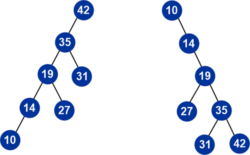

We're going to talk about AVL trees today and how they're used. The worst-case performance of BST is shown to be closest to that of linear search algorithms, i.e. O (n). We are unable to forecast data patterns and frequencies in real-time data. Therefore, the necessity to balance out the current BST emerges.

AVL trees, which stand for Adelson, Velski, and Landis, are height-balancing binary search trees. The AVL tree ensures that the height difference between the left and right sub-trees is no greater than 1. Balance Factor is the name for this.

To better grasp the distinction between balanced and unbalanced trees, let's look at some examples: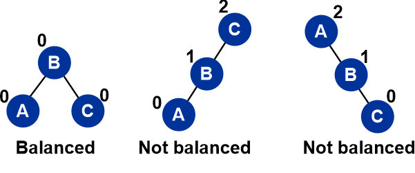

Because the height to the left and right of the root node is the same in the example above, we can see that the first tree is balanced. While the other two are not like that, the tree in the middle picture is lopsided to the left of the node. In a similar manner, the tree is lopsided to the right of the root node in the last image on the right, rendering it imbalanced.

Why use AVL Trees?

The majority of BST operations, including search, max, min, insert, delete, and others, require O(h) time, where h is the BST's height. For a skewed Binary tree, the cost of these operations can increase to O(n). We can provide an upper bound of O(log(n)) for all of these operations if we make sure that the height of the tree stays O(log(n)) after each insertion and deletion. An AVL tree's height is always O(log(n)), where n is the tree's node count.

Look at the second tree for a better understanding; C's left subtree is 2 heights tall, whereas C's right subtree is 0 heights tall, making a 2-height discrepancy. In the third tree, the difference is again 2, as the right subtree of A has height 2 and the left subtree is absent, making it height 0. Difference (balance factor) is limited to 1 by the AVL tree.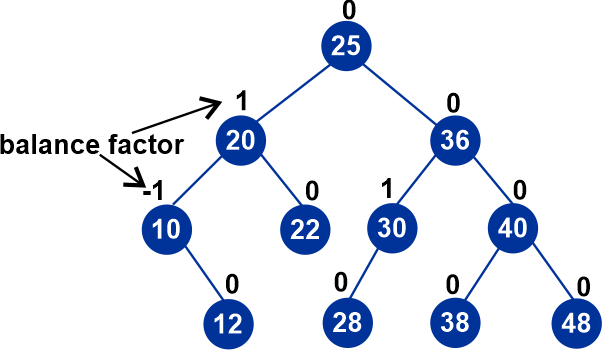

The tree is balanced using various rotational approaches if there is a height difference between the left and right sub-trees that is more than 1. To balance the AVL trees, we apply four different rotation algorithms.

Advantages of AVL Trees

• The AVL tree's height never exceeds log N, where N is the total number of nodes in the tree, since the height is always balanced.
• When compared to straightforward Binary Search trees, it provides a superior search time complexity.
• AVL trees are capable of self-balancing.

Disadvantages of AVL Trees

• The aforementioned examples show that AVL trees can be challenging to implement.
• Additionally, for particular operations, AVL trees have significant constant factors.
• Red-black trees, as opposed to AVL trees, are used in the majority of STL implementations of the ordered associative containers (sets, multisets, maps, and multimaps). Red-black trees, unlike AVL trees, only need one restructure for an insertion or removal.

We can now concentrate on AVL trees' applications since we have a better understanding of what they are, as well as their benefits and drawbacks.

Applications of AVL Trees

• Most in-memory sets and dictionaries are stored using AVL trees.
• Database applications, where insertions and deletions are less common but frequent data lookups are necessary, also frequently employ AVL trees.
• In addition to database applications, it is employed in other applications that call for better searching.
• A balanced binary search tree called an AVL tree uses rotation to keep things balanced.
• It may be used in games with plotlines as well.
• It is mostly utilized in business sectors where it is necessary to keep records on the employees that work there and their shift changes.

Conclusion

AVL trees, which were developed specifically to balance imbalanced binary trees used in database indexing, can be said to have served a specific purpose. The only difference between them and binary search trees is that in this case, we need to maintain the balance factor, which means that the data structure should remain a balanced tree as a result of various operations, which are accomplished by using the AVL tree Rotations that we previously learned about.