| |

Boltzmann MachinesBoltzmann machine refers to an association of uniformly associated neuron-like structure that make hypothetical decisions about whether to be on or off. Boltzmann Machine was invented by renowned scientist Geoffrey Hinton and Terry Sejnowski in 1985. Boltzmann Machines have a fundamental learning algorithm that permits them to find exciting features that represent complex regularities in the training data. The learning algorithm is usually slow in networks with various layers of feature detectors, but it is quick in "Restricted Boltzmann Machines" that has a single layer of feature detectors. Many hidden layers can be adapted efficiently by comprising Boltzmann Machines, utilizing the feature activations of one as the training data for the next. Boltzmann Machines are utilized to resolve two different computational issues. First, for a search problem, the weight on the associations are fixed and are used to represent a cost function. The stochastic dynamics of a Boltzmann Machine permit it to sample binary state vectors that have minimum values of the cost function. Second, for a learning issue, the Boltzmann Machine has indicated a set of binary data vectors, and this must figure out how to generate these vectors with high probability. To solve this, it must discover weights on the associations so that relative to other possible binary vectors, the data vectors have minimum values of the cost function. For solving a learning issue, Boltzmann machines make numerous small updates to their weights, and each update expects them to tackle a wide range of search issues. The Stochastic Dynamics of a Boltzmann Machine:When unit i is given a chance to update its binary state, it initially computes its absolute input, pi , which is the sum of its own bias, qi , and the weights on associations coming from other active units: Pi = qi + ?jmj wij Where, wij = It is the weight on the association between i and j, and mj is 1 when unit j is on. Unit i turns on with a probability given by the logistic function: 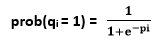
If the units are updated successively in any order that does not rely on their total inputs, the network will eventually reach a Boltzmann distribution (also known as equilibrium or stationary distribution) in which the probability of the given state vector k is determined exclusively by the "energy" of that state vector compared to the energies of all possible binary state vectors: 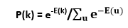
As in Hopfield networks, the energy of state vector k is defined as 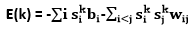
Where, sik is the binary state appointed to unit i by state vector k. If the weights on the associations are chosen so that the energies of the state vectors represent the cost of those state vector, the stochastic dynamics of a Boltzmann machine can be seen as a method for getting away from poor local optima while looking for low-cost solutions. The total input of unit i , pi , represents the difference in energy relying upon whether the units are off or on, and the way that unit i sometimes turns on even if pi is negative implies that the energy can occasionally increase during the search, therefore permitting the search to jump over energy barriers. The search can be upgraded by using simulated annealing. It scales down all of the weights and energies by a factor T, which is equivalent to the temperature of a physical network. By minimizing T from a considerable initial value to small final value, it is possible to benefit from the fast equilibrium at high temperature and still have a final equilibrium distribution that makes minimal solutions considerably more probable than high-cost ones. At a zero temperature, the update rule becomes deterministic, and a Boltzmann Machines transforms into a Hopefield network. Different types of Boltzmann Machine The learning rule can hold more complex energy functions. For example, the quadratic energy function can be replaced by an energy function that has a common term si sj sk wijk. The total input i is utilized to update rule must be replaced by 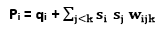
The significant change in the learning rule is that si sj is replaced by si sj sk. Boltzmann machines model the dispersion of the data vectors. However, there is a basic extension, the "conditional Boltzmann machine" for modeling conditional distributions. The significant difference between the visible and the hidden units is that when sampling (si sj) data, the visible units are clamped, and the hidden units are possibly not. If a subset of the visible units is clamped when sampling ) (si sj) model, this subset acts as "input" units, and the remaining visible units serve as "output" units. The Speed of LearningLearning is commonly very slow in Boltzmann machines with various hidden layers because the enormous networks can take quite a long time to approach their equilibrium distribution, particularly when the weights are huge and the equilibrium distribution is highly multimodal. When samples from the equilibrium distribution can be acquired, the learning signal is very noisy because it is the difference between the two sampled expectations. These issues can be overcome by confining the network, simplifying the learning algorithm, and learning one hidden layer at a time. Restricted Boltzmann Machine:The restricted Boltzmann machine invented by Smolensky in 1986. It comprises of a layer of visible units and a layer of hidden units with no visible-visible or hidden-hidden associations. With these restrictions, the hidden units are provisionally autonomous given a visible vector, so unbiased sample form (si sj) data can be obtained on one parallel step. In order to sample form (si sj)model still requires different iterations that substitute between restoring all the hidden units in parallel and restoring all the visible units in parallel. However, learning still functions well if (si sj)modelis replaced by (si sj)reconstruction , which is obtained as follows: Beginning with a data vector on the visible units, restore all of the hidden units in parallel. Update all of the visible units in parallel to obtain a reconstruction. Update all of the hidden units once again.
Next Topic#
|
 For Videos Join Our Youtube Channel: Join Now
Feedback
- Send your Feedback to [email protected]
Help Others, Please Share


