Cross Referencing in Excel

MS Excel or Microsoft Excel is a popular spreadsheet software to organize data in rows and columns. Since Excel allows users to organize vast amounts of data across multiple sheets, it allows using cells values by their references on other worksheets, same worksheets, and even in different workbooks. Cross-referencing of cells allows users to use cells' values in other cells without putting the actual values but their cell references. This can help make data calculations easier in large data sets in workbooks.

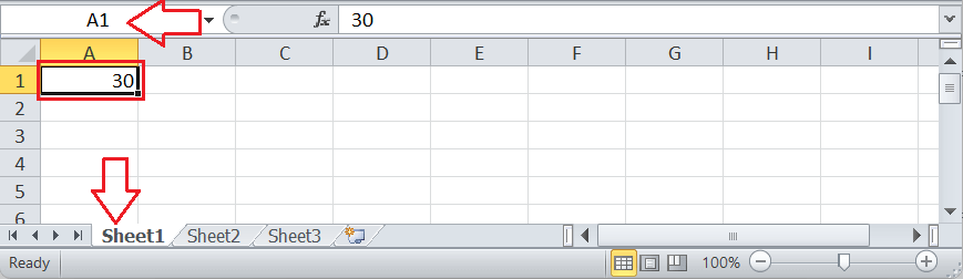
In this article, we are discussing the brief introduction of cross-referencing in Excel. This article also discusses the step-by-step process of cross-referencing in different scenarios, including the example.

What is Cross Referencing in Excel?

Each cell in Excel workbook is represented by a unique address, known as a cell reference. The cell reference is typically the combination of specific column and row addresses. It consists of the letter representing the respective cell's column and the number representing the corresponding row. In the Excel workbook, the same position cells in different sheets represent identical cell references.

Cross-reference is nothing but a reference to information located somewhere else in the same Excel workbook. To cross-reference between different workbook sheets, we must know about identifying cells by their extended addresses. The extended references help us specify the exact cell, including its sheet name, column, and row.

Let us understand the cross-referencing with a simple example where we will be using the first cell of the worksheet for cross-referencing:

• First, we must identify the cell's column that we wish to apply to cross-reference. For example, the first cell in an Excel sheet is a part of column A.
  
• Next, we must identify the row to which the corresponding cell belongs. For example, the first cell in an Excel sheet is a part of the first row.
  
• We need to combine both the above points to form the cell address for the first cell on the worksheet. Thus, when we combine characters for column and row, the cell address for the first cell becomes 'A1'.
  
• After that, we need to identify the corresponding sheet name. The default names for cells' sheet are 'Sheet1', 'Sheet2', 'Sheet3', etc. In our example, it is 'Sheet1'.
  
• We must append the sheet name to the identified cell address, separated by the exclamation mark, to identify the extended reference for the specific cell. In our example, the first cell of the worksheet belongs to the following extended reference: "Sheet1!A1".
  
• Suppose we have the numerical value (30) in the first cell of Sheet1 that we want to sum up with another numerical value (20) and get the result in the first cell of Sheet2 of our workbook. Thus, we have to use the extended reference of the first cell of the first sheet in the first cell of the second sheet and append the formula like this: "=Sheet1!A1 + 20", without quotes.
  
  In the above image, we can see that the values are added from the different sheets of the workbook using cross-referencing.

How to cross-reference cells in Excel?

Based on the scenarios, there can be different ways we may need to use cross reference in Excel. The following are the most typical cross-referencing methods used in Excel sheets:

• Cross Referencing Single Cells in Excel
• Referencing Cell Ranges in Excel
• Referencing Named Cells in Excel

Let us now understand each in detail:

Cross Referencing Single Cells in Excel

In a location map, the idea of grid references is used. The map is split up into various grids that help us pinpoint any particular location on the map. We typically specify any location on a map by using the individual grid references. In Excel, the spreadsheets work in an almost similar way.

An Excel spreadsheet contains various cells that we can specify by their individual references, created by combining a letter for the corresponding column and a number for a specific row. For example, cell B4 is in the grid that intersects the second column (column B) and row 4. Suppose that B4 is a cell in our workbook Book1.xlsx.

To reference B4 in any other cell within the same sheet, we must enter =B4 into the resultant cell. Also, we can type any desired formula with multiple cell references to get results combining values from different cells. For instance, we can type "=B4*B5" without quotes to multiply the data from cell B4 and cell B5 on any other cell, as shown below:

After putting the formula combining the cell references, we must press the Enter key to get the resultant value. The above formula in the above provides the following result: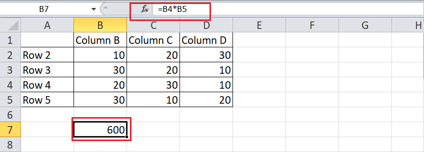

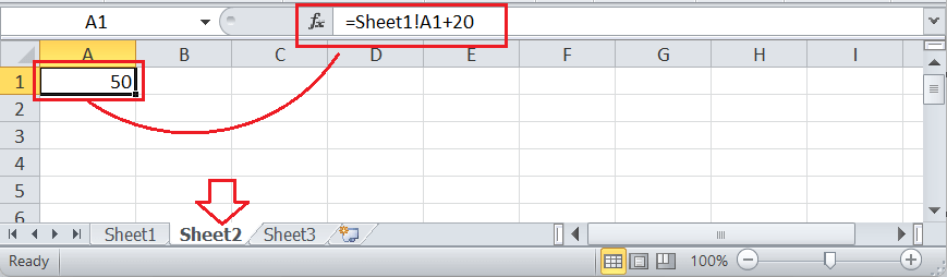
In this way, we can use cross-referencing with single cells in the same worksheet. However, to reference a cell from another sheet, we must append the worksheet name before the cell, followed by the exclamation mark. For instance, if we use the formula =Sheet1!B4*Sheet2!B5 in any cell of the Sheet2, we will get the same result as above (i.e., 600). The corresponding formula will multiply the values from cells B4 and B5 from Sheet1 and provide the resultant value in the selected cell of Sheet2.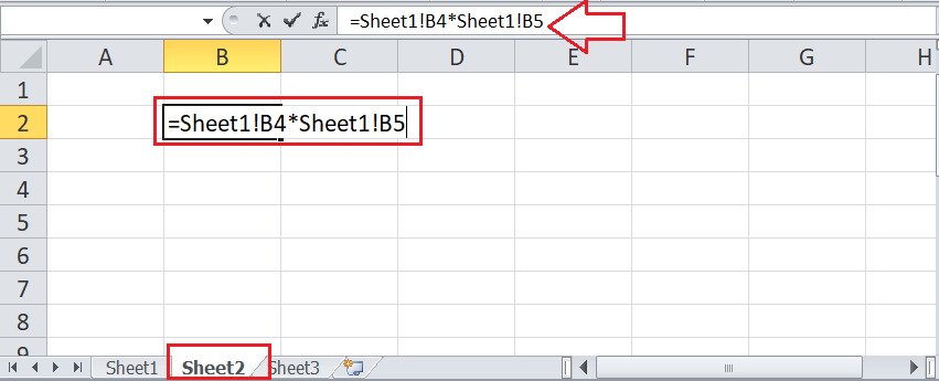

After pressing the Enter key, the result is the same: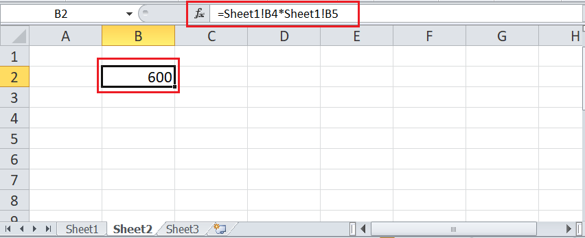

In this way, we can use cross-referencing with single cells in different worksheets. Besides, Excel also allows us to reference cells from another workbook (Excel file). For this, we must use the square brackets to specify the specific Excel workbook name, followed by the extended reference. For example, =[Book1.xlsx]Sheet2!B2 will represent the same value (600) as shown in the above image when used in another workbook of the same folder.

Suppose we create a new Excel file (Book2.xlsx) in the same folder as our above file (Book1.xlsx) exists. Then in Book2.xlsx, we apply the formula =[Book1.xlsx]Sheet1!B4*[Book1.xlsx]Sheet1!B5 in any cell, as shown below: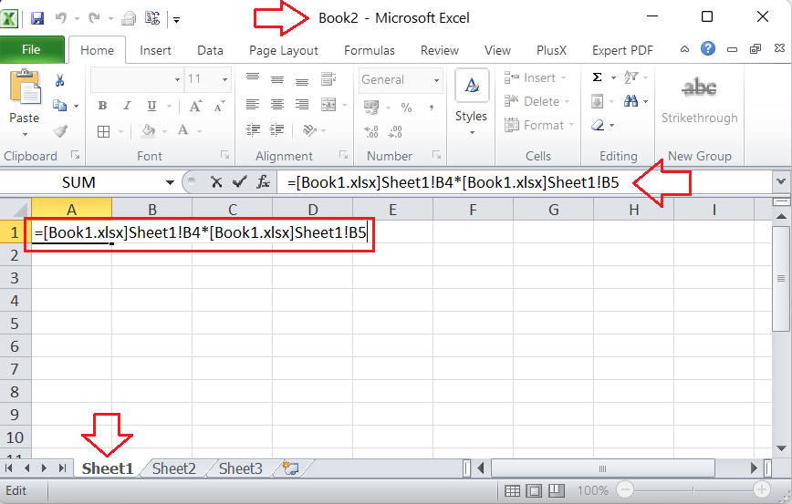

After pressing the Enter key, the resultant value is given by multiplying the values from cells B4 and B5 from the Sheet1 of Excel workbook Book1.xlsx.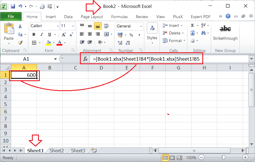

In this way, we can use references in Excel for individual cells in the same sheet, different sheets, and even different workbooks/ spreadsheets.

Referencing Cell Ranges in Excel

Excel also allows users to apply specific formulae by referencing multiple cells if the cells are in sequential order. In such cases, we can use the entire cell ranges in corresponding formulae.

For example, when we need to sum values in cells B3 to B7 in our example workbook (Book1.xlsx), we usually take the entire range and supply it in a formula like this: =SUM(B3:B7). This means that we specify the range by using a colon and connecting the start and end cells.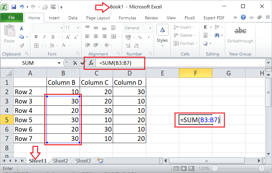

After typing the formula, we must press the Enter key to get the resultant value, as shown below: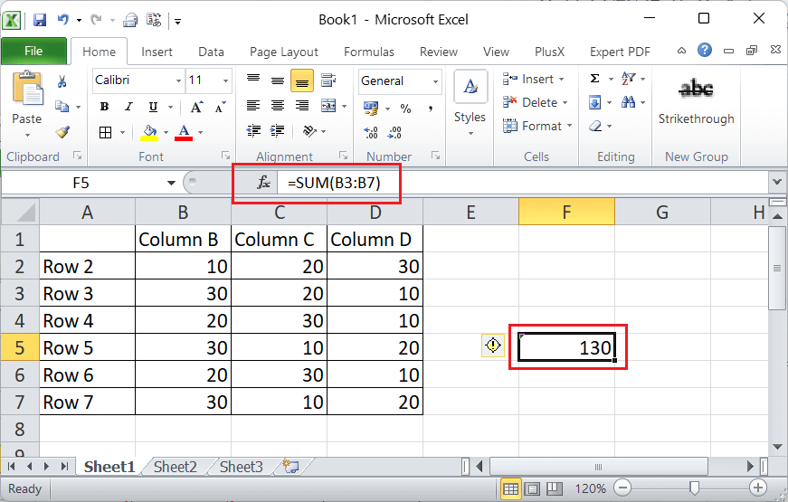

We can use the cell ranges in other sheets and workbooks by their references. The method is almost the same as the referencing approach we discussed above for individual cells.

When we need to reference a cell range in another sheet within the same workbook, we must specify the corresponding sheet name before the cell range. For example, to find the sum of cells B3 to B7 from the Sheet1 into any desired cell in Sheet2, we can use the formula like this: =SUM(Sheet1!B3:B7).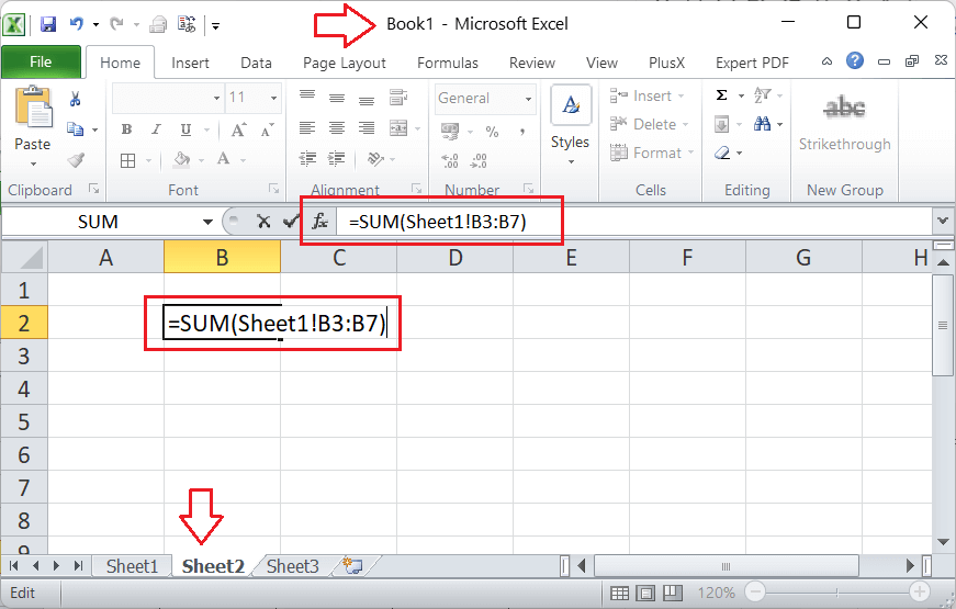

After pressing the Enter key, we get the resultant value in the Sheet2, the same as the above resultant sum we calculated in the Sheet1.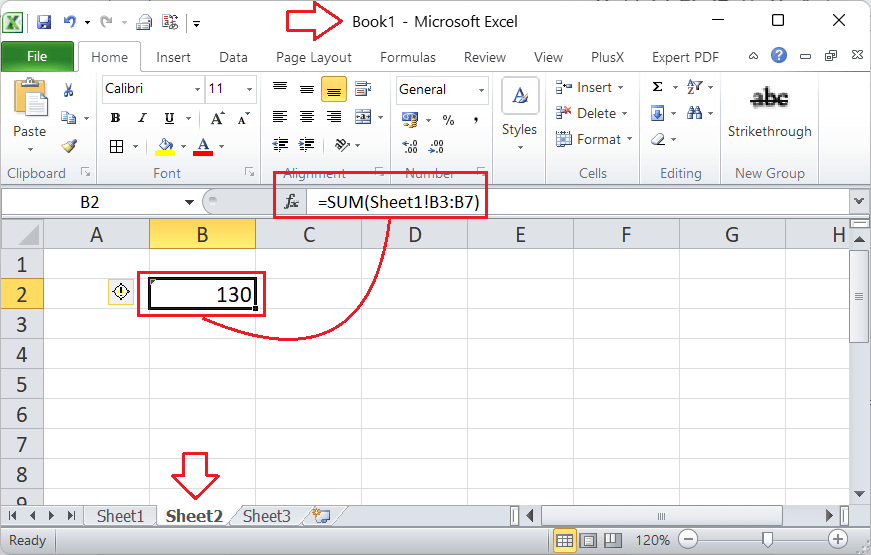

When referencing a cell range from different Excel workbook, we need to type square brackets and the corresponding file name inside the box, followed by the extended reference and the cell range. Suppose we need to sum up the value from cells B3 to B7 and get the resultant value in any cell of another Excel file (Book2.xlsx) that is in the same folder as our primary file (Book1.xlsx) exists. Then in Book2.xlsx, we need to apply the formula =SUM([Book1.xlsx]Sheet1!B3:B7) in any cell, as shown below: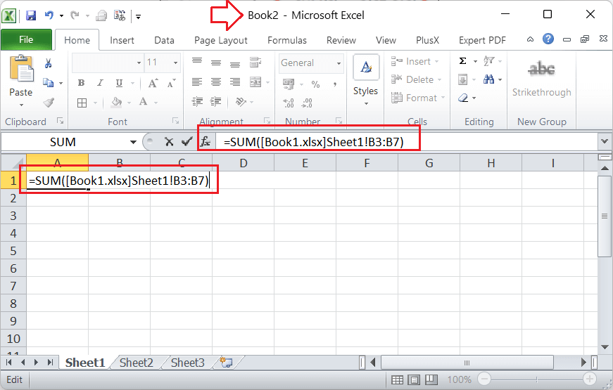

After pressing the Enter key, the resultant value is given in another workbook (Book2.xlsx) by adding the values in cells B3 to B7 from the Sheet1 of primary Excel workbook (Book1.xlsx).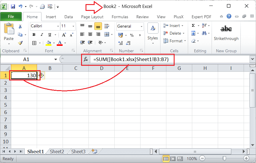

In this way, we can use references in Excel for a range of cells in the same sheet, different sheets, and even different workbooks or spreadsheets.

Referencing Named Cells in Excel

Excel allows users to specify any particular name to the desired cell within the spreadsheet. It helps to ease the referencing approach by replacing the grid-style referencing method and allows using the specific name for a particular cell simplifies referencing cell and cell ranges.

For instance, if we name a cell as 'data', we can use this name as a reference throughout the entire workbook for a defined cell. We don't need to define the extended reference in that case. This typically eliminates the chances of mistyping a cell reference or cell range and saves potential time.

To specify the desired name to any cell in the workbook, we need to select or highlight the particular cell, press the right-click button, and select the 'Define Name' option. It looks like this: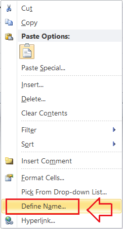

In the next window, we need to type the name for the selected cell, select the scope to use the typed name for the entire workbook or specific sheets, and click the OK button.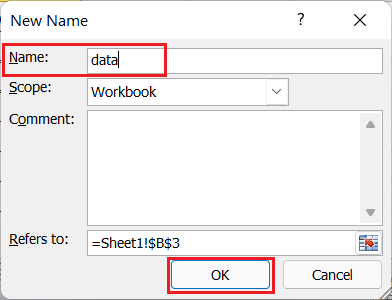

After saving the name, we can click on the particular cell and see its name in the reference area. We can also use the naming approach to define a name for a specific range of cells.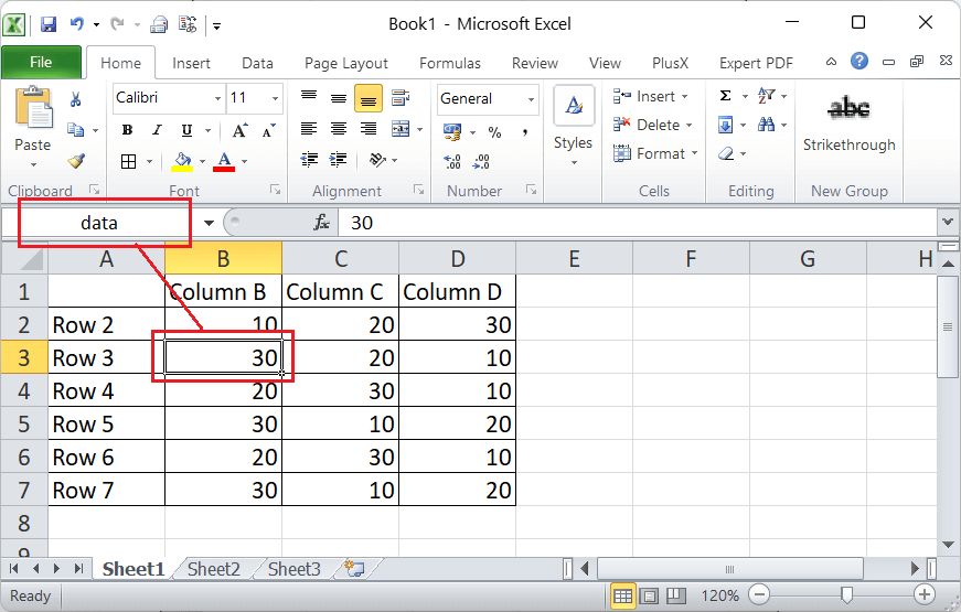

After defining a name, we can use it as a reference using the formula: =data.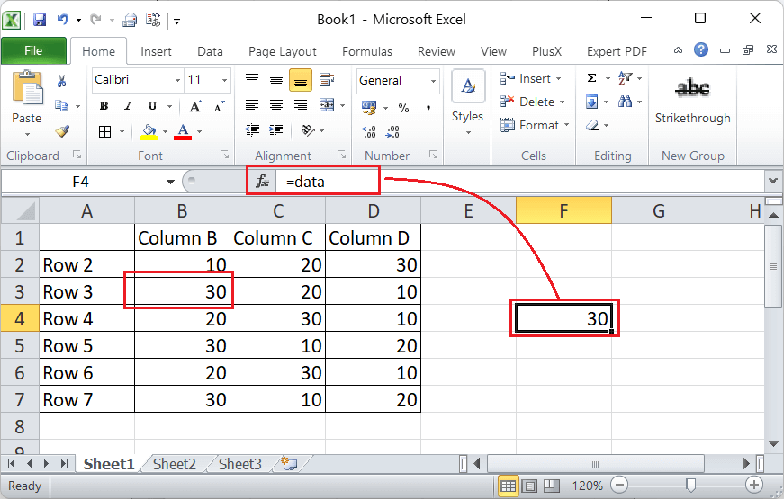

Since we selected the 'workbook' option as a scope while naming the cell, the named cell reference can also be used in other workbook sheets. For instance, if we use the same formula (=data) in the Sheet2, we will get the same result, as shown below: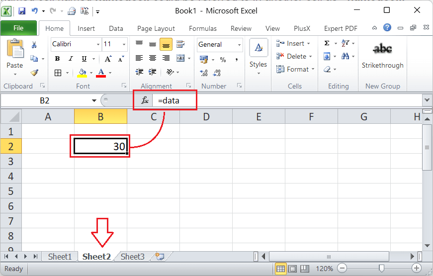

Suppose we want to reference a named cell in another Excel workbook. We don't need to use the square box to type a specific workbook name inside it. Instead, we can easily specify the corresponding Excel workbook name, followed by the exclamation mark and the named cell.

For instance, we can enter the formula '=Book1.xlsx!data' without quotes in any specific cell of another workbook (Book2.xlsx) and get the same result as we achieved in the above image. But, the workbooks must be saved in the same folder.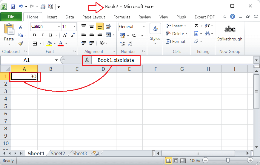

In this way, we can use references in Excel for named cells in the same sheet, different sheets, and even different workbooks or spreadsheets.

Example of Cross-Referencing using VLOOKUP

When we have data in multiple lists, it is not easy to manually keep all the data together in one list. However, we can cross-reference them using vlookup. It does not matter how long our data list is; we can do hundreds or thousands of cross-references with a few clicks.

VlookUp searches for the values vertically down for the supplied table. The syntax of this function is as follows:

Where the four parameters are as below:

• lookup_value: It is user input. We give this value to the function to search on to use cross-reference to the other list.
• table_array: It is the range of cells where the table is located. It mainly contains the column that is being searched on and the data columns for which we will get the values we want.
• col_index_num: It is a column of data that has the answer we want.
• range_lookup: This value can be either TRUE or FALSE. When it is set to TRUE, the function provides the closest result to the lookup value without looking further. On the other hand, when it is set to FALSE, the lookup function gives the exact match if found; otherwise, it returns #N/A.

Let us now cross-reference data between two Excel sheets:

Suppose we have the following sheet with some employees' IDs, names, and dates of birth.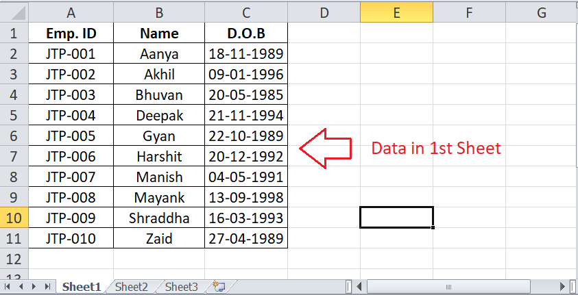

Also, we have another sheet with almost the same employees and their favorite colors.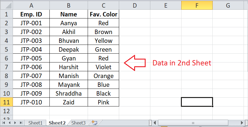

We need to create a combined list from both the above sheets to display employees' IDs, names, their dates of birth and favourite colors in the same sheet. We must use the VLOOKUP by using the following data in a new column (Fav. Color) created in the Sheet1:

• The lookup value in our example is the employees' names list.
• The table array is the table in the second sheet from cells B2 to B11.
• The column index is the answer we need. In our example, it is the column with favorite colors. Thus, the column index number is 2 (2^nd column of the supplied table array).
• Since we want to get the exact matches, we will use FALSE as the fourth parameter.

After applying VLOOKUP with the above values, we will get the desired results like this: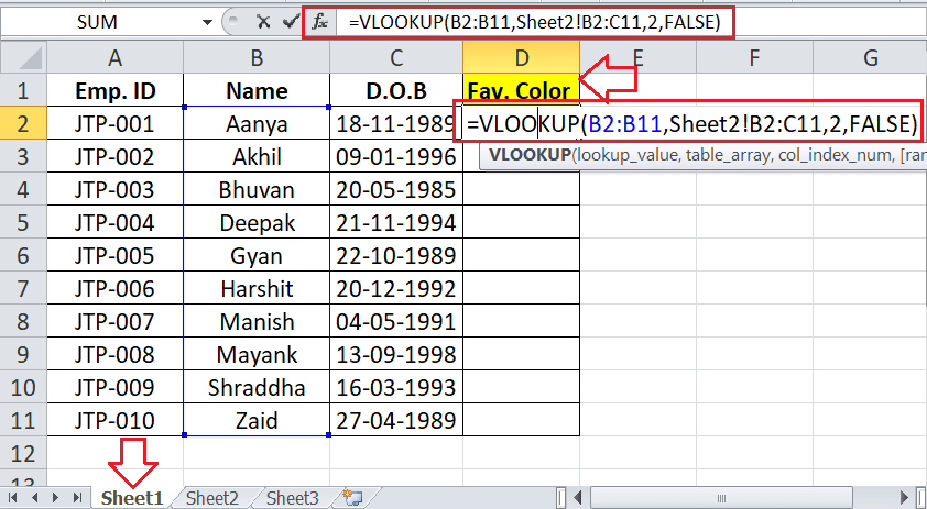

After pressing the Enter key and copying (or dragging) the formula into other cells, we get the following results: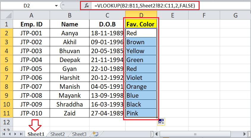

In the above image, the VLOOKUP function has searched for colors from Sheet2 and provided the results in Sheet1. This is the most common example of cross-referencing in Excel.