Data Preprocessing in Machine learning

Data preprocessing is a process of preparing the raw data and making it suitable for a machine learning model. It is the first and crucial step while creating a machine learning model.

When creating a machine learning project, it is not always a case that we come across the clean and formatted data. And while doing any operation with data, it is mandatory to clean it and put in a formatted way. So for this, we use data preprocessing task.

Why do we need Data Preprocessing?

A real-world data generally contains noises, missing values, and maybe in an unusable format which cannot be directly used for machine learning models. Data preprocessing is required tasks for cleaning the data and making it suitable for a machine learning model which also increases the accuracy and efficiency of a machine learning model.

It involves below steps:

• Getting the dataset
• Importing libraries
• Importing datasets
• Finding Missing Data
• Encoding Categorical Data
• Splitting dataset into training and test set
• Feature scaling

1) Get the Dataset

To create a machine learning model, the first thing we required is a dataset as a machine learning model completely works on data. The collected data for a particular problem in a proper format is known as the dataset.

Dataset may be of different formats for different purposes, such as, if we want to create a machine learning model for business purpose, then dataset will be different with the dataset required for a liver patient. So each dataset is different from another dataset. To use the dataset in our code, we usually put it into a CSV file. However, sometimes, we may also need to use an HTML or xlsx file.

What is a CSV File?

CSV stands for "Comma-Separated Values" files; it is a file format which allows us to save the tabular data, such as spreadsheets. It is useful for huge datasets and can use these datasets in programs.

Here we will use a demo dataset for data preprocessing, and for practice, it can be downloaded from here, "https://www.superdatascience.com/pages/machine-learning. For real-world problems, we can download datasets online from various sources such as https://www.kaggle.com/uciml/datasets, https://archive.ics.uci.edu/ml/index.php etc.

We can also create our dataset by gathering data using various API with Python and put that data into a .csv file.

2) Importing Libraries

In order to perform data preprocessing using Python, we need to import some predefined Python libraries. These libraries are used to perform some specific jobs. There are three specific libraries that we will use for data preprocessing, which are:

Numpy: Numpy Python library is used for including any type of mathematical operation in the code. It is the fundamental package for scientific calculation in Python. It also supports to add large, multidimensional arrays and matrices. So, in Python, we can import it as:

Here we have used nm, which is a short name for Numpy, and it will be used in the whole program.

Matplotlib: The second library is matplotlib, which is a Python 2D plotting library, and with this library, we need to import a sub-library pyplot. This library is used to plot any type of charts in Python for the code. It will be imported as below:

Here we have used mpt as a short name for this library.

Pandas: The last library is the Pandas library, which is one of the most famous Python libraries and used for importing and managing the datasets. It is an open-source data manipulation and analysis library. It will be imported as below:

Here, we have used pd as a short name for this library. Consider the below image: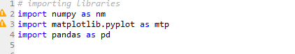

3) Importing the Datasets

Now we need to import the datasets which we have collected for our machine learning project. But before importing a dataset, we need to set the current directory as a working directory. To set a working directory in Spyder IDE, we need to follow the below steps:

1. Save your Python file in the directory which contains dataset.
2. Go to File explorer option in Spyder IDE, and select the required directory.
3. Click on F5 button or run option to execute the file.

Note: We can set any directory as a working directory, but it must contain the required dataset.

Here, in the below image, we can see the Python file along with required dataset. Now, the current folder is set as a working directory.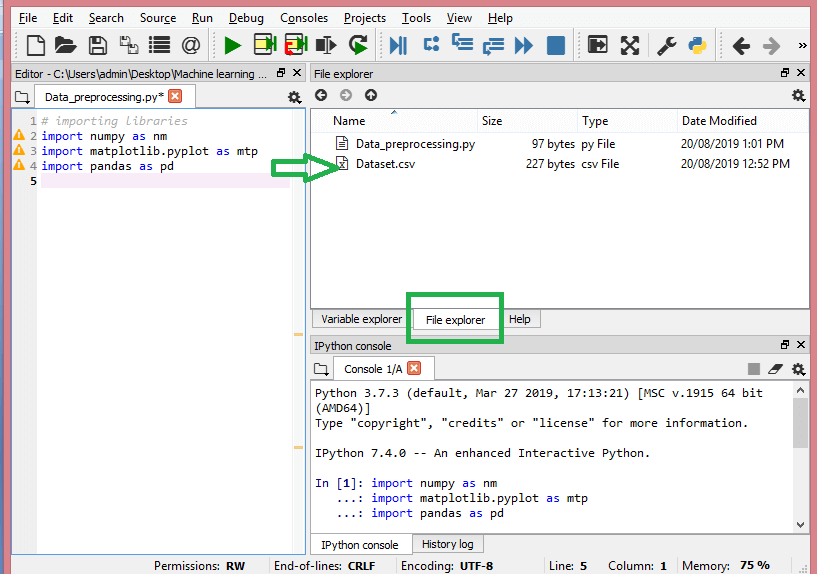

read_csv() function:

Now to import the dataset, we will use read_csv() function of pandas library, which is used to read a csv file and performs various operations on it. Using this function, we can read a csv file locally as well as through an URL.

We can use read_csv function as below:

Here, data_set is a name of the variable to store our dataset, and inside the function, we have passed the name of our dataset. Once we execute the above line of code, it will successfully import the dataset in our code. We can also check the imported dataset by clicking on the section variable explorer, and then double click on data_set. Consider the below image: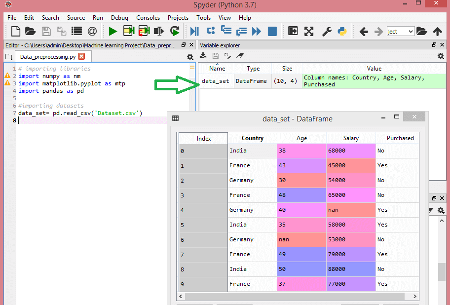

As in the above image, indexing is started from 0, which is the default indexing in Python. We can also change the format of our dataset by clicking on the format option.

Extracting dependent and independent variables:

In machine learning, it is important to distinguish the matrix of features (independent variables) and dependent variables from dataset. In our dataset, there are three independent variables that are Country, Age, and Salary, and one is a dependent variable which is Purchased.

Extracting independent variable:

To extract an independent variable, we will use iloc[ ] method of Pandas library. It is used to extract the required rows and columns from the dataset.

In the above code, the first colon(:) is used to take all the rows, and the second colon(:) is for all the columns. Here we have used :-1, because we don't want to take the last column as it contains the dependent variable. So by doing this, we will get the matrix of features.

By executing the above code, we will get output as:

As we can see in the above output, there are only three variables.

Extracting dependent variable:

To extract dependent variables, again, we will use Pandas .iloc[] method.

Here we have taken all the rows with the last column only. It will give the array of dependent variables.

By executing the above code, we will get output as:

Output:

array(['No', 'Yes', 'No', 'No', 'Yes', 'Yes', 'No', 'Yes', 'No', 'Yes'],
      dtype=object)

Note: If you are using Python language for machine learning, then extraction is mandatory, but for R language it is not required.

4) Handling Missing data:

The next step of data preprocessing is to handle missing data in the datasets. If our dataset contains some missing data, then it may create a huge problem for our machine learning model. Hence it is necessary to handle missing values present in the dataset.

Ways to handle missing data:

There are mainly two ways to handle missing data, which are:

By deleting the particular row: The first way is used to commonly deal with null values. In this way, we just delete the specific row or column which consists of null values. But this way is not so efficient and removing data may lead to loss of information which will not give the accurate output.

By calculating the mean: In this way, we will calculate the mean of that column or row which contains any missing value and will put it on the place of missing value. This strategy is useful for the features which have numeric data such as age, salary, year, etc. Here, we will use this approach.

To handle missing values, we will use Scikit-learn library in our code, which contains various libraries for building machine learning models. Here we will use Imputer class of sklearn.preprocessing library. Below is the code for it:

Output:

array([['India', 38.0, 68000.0],
       ['France', 43.0, 45000.0],
       ['Germany', 30.0, 54000.0],
       ['France', 48.0, 65000.0],
       ['Germany', 40.0, 65222.22222222222],
       ['India', 35.0, 58000.0],
       ['Germany', 41.111111111111114, 53000.0],
       ['France', 49.0, 79000.0],
       ['India', 50.0, 88000.0],
       ['France', 37.0, 77000.0]], dtype=object

As we can see in the above output, the missing values have been replaced with the means of rest column values.

5) Encoding Categorical data:

Categorical data is data which has some categories such as, in our dataset; there are two categorical variable, Country, and Purchased.

Since machine learning model completely works on mathematics and numbers, but if our dataset would have a categorical variable, then it may create trouble while building the model. So it is necessary to encode these categorical variables into numbers.

For Country variable:

Firstly, we will convert the country variables into categorical data. So to do this, we will use LabelEncoder() class from preprocessing library.

Output:

Out[15]: 
  array([[2, 38.0, 68000.0],
            [0, 43.0, 45000.0],
         [1, 30.0, 54000.0],
         [0, 48.0, 65000.0],
         [1, 40.0, 65222.22222222222],
         [2, 35.0, 58000.0],
         [1, 41.111111111111114, 53000.0],
         [0, 49.0, 79000.0],
         [2, 50.0, 88000.0],
        [0, 37.0, 77000.0]], dtype=object)

Explanation:

In above code, we have imported LabelEncoder class of sklearn library. This class has successfully encoded the variables into digits.

But in our case, there are three country variables, and as we can see in the above output, these variables are encoded into 0, 1, and 2. By these values, the machine learning model may assume that there is some correlation between these variables which will produce the wrong output. So to remove this issue, we will use dummy encoding.

Dummy Variables:

Dummy variables are those variables which have values 0 or 1. The 1 value gives the presence of that variable in a particular column, and rest variables become 0. With dummy encoding, we will have a number of columns equal to the number of categories.

In our dataset, we have 3 categories so it will produce three columns having 0 and 1 values. For Dummy Encoding, we will use OneHotEncoder class of preprocessing library.

Output:

array([[0.00000000e+00, 0.00000000e+00, 1.00000000e+00, 3.80000000e+01,
        6.80000000e+04],
       [1.00000000e+00, 0.00000000e+00, 0.00000000e+00, 4.30000000e+01,
        4.50000000e+04],
       [0.00000000e+00, 1.00000000e+00, 0.00000000e+00, 3.00000000e+01,
        5.40000000e+04],
       [1.00000000e+00, 0.00000000e+00, 0.00000000e+00, 4.80000000e+01,
        6.50000000e+04],
       [0.00000000e+00, 1.00000000e+00, 0.00000000e+00, 4.00000000e+01,
        6.52222222e+04],
       [0.00000000e+00, 0.00000000e+00, 1.00000000e+00, 3.50000000e+01,
        5.80000000e+04],
       [0.00000000e+00, 1.00000000e+00, 0.00000000e+00, 4.11111111e+01,
        5.30000000e+04],
       [1.00000000e+00, 0.00000000e+00, 0.00000000e+00, 4.90000000e+01,
        7.90000000e+04],
       [0.00000000e+00, 0.00000000e+00, 1.00000000e+00, 5.00000000e+01,
        8.80000000e+04],
       [1.00000000e+00, 0.00000000e+00, 0.00000000e+00, 3.70000000e+01,
        7.70000000e+04]])

As we can see in the above output, all the variables are encoded into numbers 0 and 1 and divided into three columns.

It can be seen more clearly in the variables explorer section, by clicking on x option as: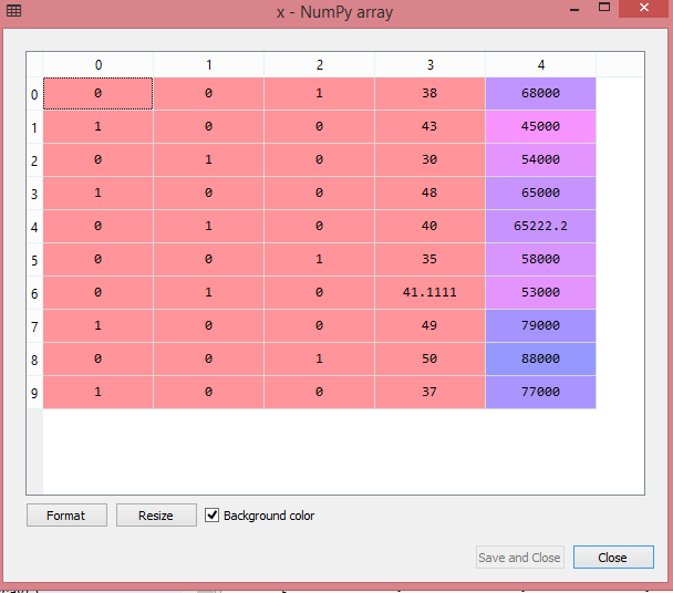

For Purchased Variable:

For the second categorical variable, we will only use labelencoder object of LableEncoder class. Here we are not using OneHotEncoder class because the purchased variable has only two categories yes or no, and which are automatically encoded into 0 and 1.

Output:

Out[17]: array([0, 1, 0, 0, 1, 1, 0, 1, 0, 1])

It can also be seen as: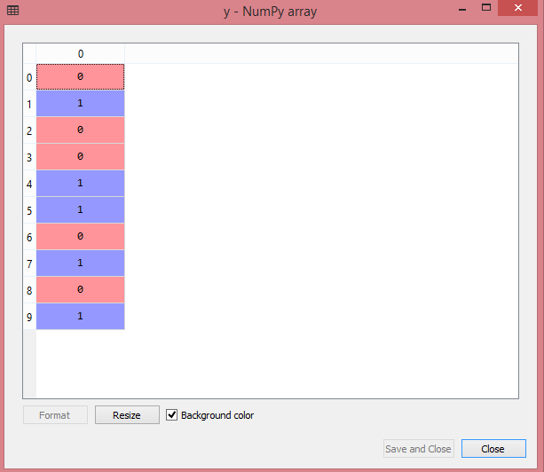

6) Splitting the Dataset into the Training set and Test set

In machine learning data preprocessing, we divide our dataset into a training set and test set. This is one of the crucial steps of data preprocessing as by doing this, we can enhance the performance of our machine learning model.

Suppose, if we have given training to our machine learning model by a dataset and we test it by a completely different dataset. Then, it will create difficulties for our model to understand the correlations between the models.

If we train our model very well and its training accuracy is also very high, but we provide a new dataset to it, then it will decrease the performance. So we always try to make a machine learning model which performs well with the training set and also with the test dataset. Here, we can define these datasets as: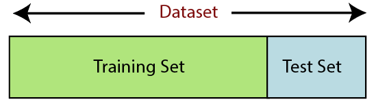

Training Set: A subset of dataset to train the machine learning model, and we already know the output.

Test set: A subset of dataset to test the machine learning model, and by using the test set, model predicts the output.

For splitting the dataset, we will use the below lines of code:

Explanation:

• In the above code, the first line is used for splitting arrays of the dataset into random train and test subsets.
• In the second line, we have used four variables for our output that are
  • x_train: features for the training data
  • x_test: features for testing data
  • y_train: Dependent variables for training data
  • y_test: Independent variable for testing data
• In train_test_split() function, we have passed four parameters in which first two are for arrays of data, and test_size is for specifying the size of the test set. The test_size maybe .5, .3, or .2, which tells the dividing ratio of training and testing sets.
• The last parameter random_state is used to set a seed for a random generator so that you always get the same result, and the most used value for this is 42.

Output:

By executing the above code, we will get 4 different variables, which can be seen under the variable explorer section.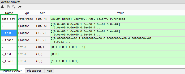

As we can see in the above image, the x and y variables are divided into 4 different variables with corresponding values.

7) Feature Scaling

Feature scaling is the final step of data preprocessing in machine learning. It is a technique to standardize the independent variables of the dataset in a specific range. In feature scaling, we put our variables in the same range and in the same scale so that no any variable dominate the other variable.

Consider the below dataset: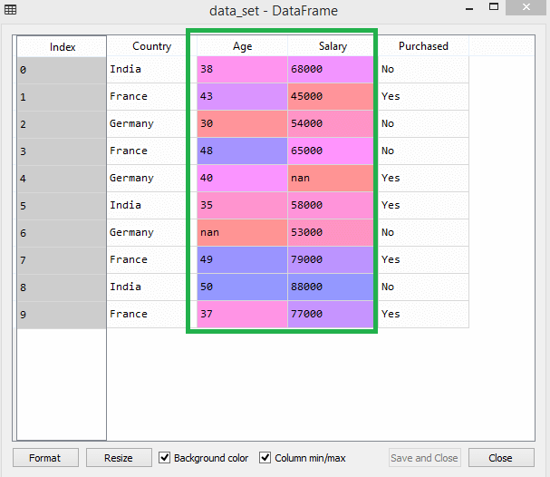

As we can see, the age and salary column values are not on the same scale. A machine learning model is based on Euclidean distance, and if we do not scale the variable, then it will cause some issue in our machine learning model.

Euclidean distance is given as: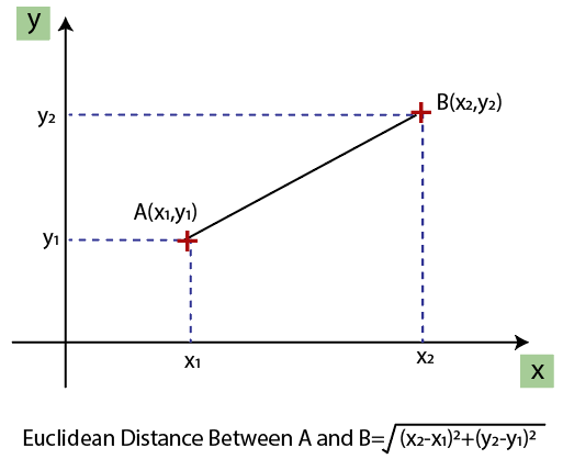

If we compute any two values from age and salary, then salary values will dominate the age values, and it will produce an incorrect result. So to remove this issue, we need to perform feature scaling for machine learning.

There are two ways to perform feature scaling in machine learning:

Standardization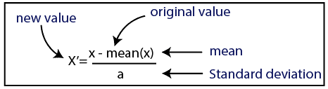

Normalization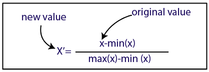

Here, we will use the standardization method for our dataset.

For feature scaling, we will import StandardScaler class of sklearn.preprocessing library as:

Now, we will create the object of StandardScaler class for independent variables or features. And then we will fit and transform the training dataset.

For test dataset, we will directly apply transform() function instead of fit_transform() because it is already done in training set.

Output:

By executing the above lines of code, we will get the scaled values for x_train and x_test as:

x_train: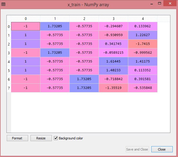

x_test: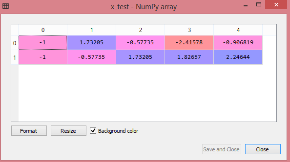

As we can see in the above output, all the variables are scaled between values -1 to 1.

Note: Here, we have not scaled the dependent variable because there are only two values 0 and 1. But if these variables will have more range of values, then we will also need to scale those variables.

Combining all the steps:

Now, in the end, we can combine all the steps together to make our complete code more understandable.

In the above code, we have included all the data preprocessing steps together. But there are some steps or lines of code which are not necessary for all machine learning models. So we can exclude them from our code to make it reusable for all models.