Dynamic Named Range

What is called Dynamic Named Range?

As the name suggests, a range is created dynamically to automatically accommodate or accept new values. In a dynamic named range, the reference reacts to the changes. If a new value is added to the list, it expands in the default manner. Suppose a particular value is deleted or removed from the list. Automatically, the list contracts. The reference or formula in the dynamic named range may vary based on the user input or value in another cell. Creating a Dynamic Named range for the list or data helps save the edited data changes. Here in this tutorial, the various methods of creating dynamic named ranges are explained briefly.

Some of the examples of the dynamic named range are as follows,

Example 1: Create a dynamic named range for given data

Here in this example, the step-by-step process of creating a dynamic named range is explained briefly.

Step 1: Enter the required data in the worksheet, namely A1:A5.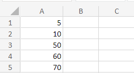

Step 2.1: To create a dynamic named range, first create the named range for the respective data. Naming the range helps the user to address the range name in the formula more quickly and easily. Moreover, the formula identifies the range easily.

Step 2.2: Select the data present in the worksheet. Choose Define Name from the Define Name group in the formula tab.

Step 2.3: The New Name dialog box will appear. In that, enter the name of the data in the Name box. The selected range will appear in the 'Refers to' section.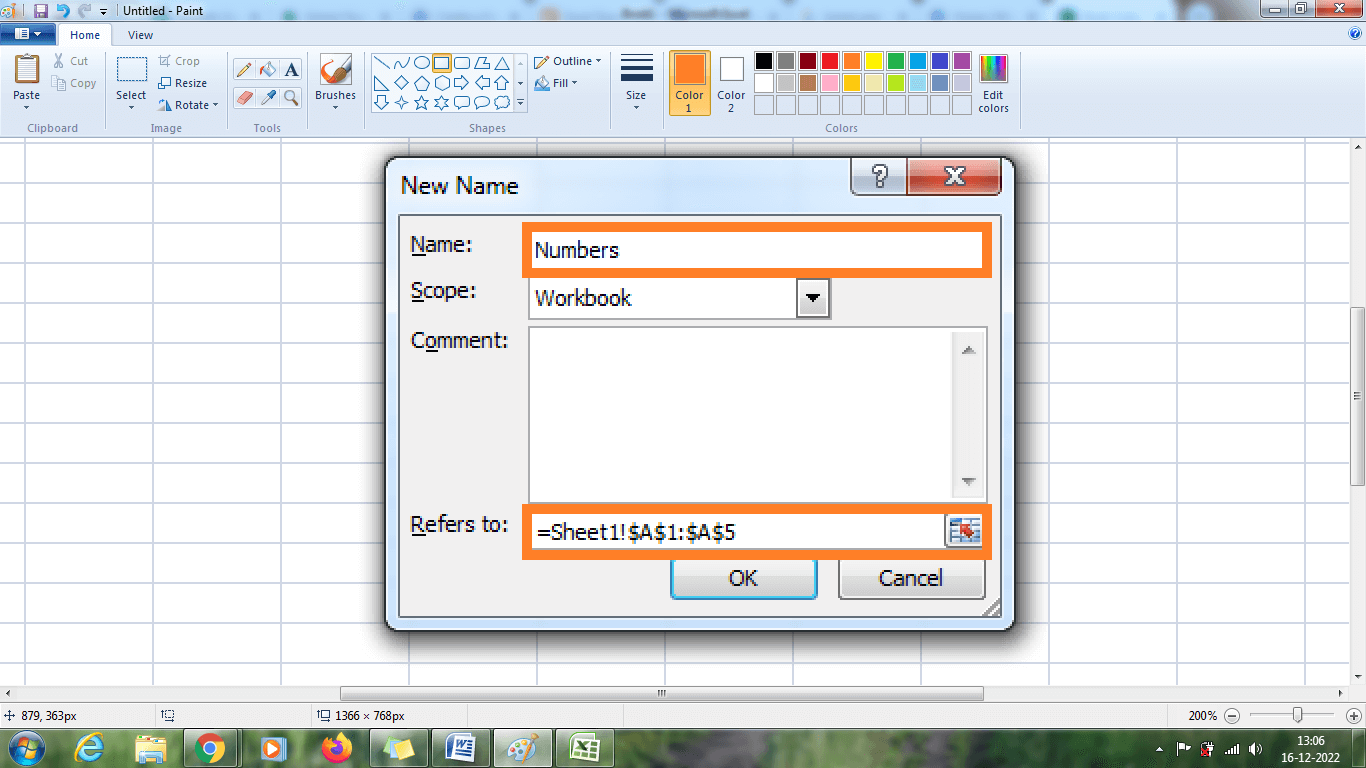

Step 2.4: Here in this worksheet, the range is named Numbers. The named range is created for the given data. After entering the data, Press Enter.

Another alternative way to create the named range quickly is as follows,

Select the respective range in the data, and type the range name in the Name box. Press Enter and the named range is created for the data.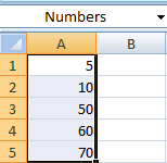

By naming 'Numbers,' the range is created.

Step 3: To sum the named range, select a new cell and enter the formula as =SUM (Numbers).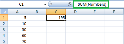

From the worksheet, the SUM function calculates the sum value for given data.

Step 4: For example, if a new value is added to the data, excel won't update the new data. The result remains the same.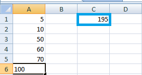

From the above worksheet, the new value called 100 is added, where the result remains the same.

Step 5: A dynamic named range is created to update the new data in the named range automatically.

Step 6: Click Name Manager in the Defined Names Group in the formula tab. The Name Manager Dialog box will display. In that, choose the Edit option.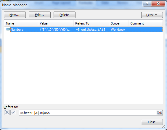

Step 7: The Edit Name dialog box will display. In Refers to section, type the formula as =OFFSET ($A$1, 0, 0, COUNTA ($A: $A), 1).

Step 8: Press OK. The result present in cell C1 automatically updates to the new values.

STEP 9: In the formula, the OFFSET function contains five arguments. Here $A$1 is called a reference, rows to offset -0, columns to offset-0, COUNTA ($A: $A) is called height, and width is called 1. The COUNTA ($A: $A) counts the value present in the column, and if a new value is added, the COUNTA ($A: $A) increases. Hence the OFFSET function expands.

Step 10: Now, add any value to column A. It automatically updates the result in the selected cell.

OFFSET Function

One of the familiar functions is called the OFFSET function, which is used to create a dynamic named range. This function denotes the range with a selective number of rows and columns starting with the reference cell.

Syntax

Here in the formula,

Reference - Reference in the formula indicates which the user wants to base the offset. It refers to the cell or adjacent cells.

Rows- The number of rows is required, whether up or down, where the user wants the upper-left cell to be referred to. For example, if 5 a row argument indicates that the five rows are below the reference.

Column- The column number indicates where the user wants the upper left cell of the result to be referred to. If the column number is positive, it indicates the right of the starting reference, and if it is negative, it indicates the left of the starting reference. For example, if 5 a column argument, the upper left cell in the reference is five columns to the right of the reference.

Height- The value of height must be positive. It is an optional one where it indicates the returned reference to be.

Width- The width value must be positive, which refers to several columns. It is an optional one where it indicates the returned reference to be.

What is the need for the OFFSET function in Excel?

There is a question: Why does it need an OFFSET function? Because simply writing the direct cell reference is easier. For the following reason, the OFFSET function is used,

To create dynamic ranges- For example, writing the cell reference A1:B5 is static, and it is easier to perform some tasks. Sometimes change in the data will occur, like new column or rows is added frequently in the worksheet.

Address of the range- Sometimes, the address of the range is not known. Hence OFFSET function is used.

Here is an example of the OFFSET function,

Example 2: Sum the data in the cell where new data is added every week.

Here in this example, the data contains the Month name and bonus per month. In the source data, every new data is added above the Total value. Either the user updates the total manually in the SUM formula or uses the OFFSET function. The OFFSET function is used to summarize the data because new data is added every month. The steps to be followed are,

Step 1: Enter the data in the worksheet, namely A1:B7, namely month and bonus.

Step 2: To sum the data up to B7, select a new cell called Total and enter the formula as =SUM (B2:B7). The result will be displayed as shown below,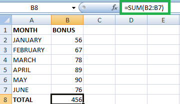

Step 3: If a new value is added to the list every month, how to sum the values. Here OFFSET function is used. For example, if a new value is added in cell B8 the formula will be like = SUM (B2 :( OFFSET (B9,-1, 0))). Here in the formula, B9 is called cell reference, -1 indicates right above the total value, and '0' is called column number, as there is no need to change the column number.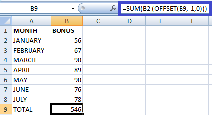

From the above worksheet, the new value will be added automatically by using the OFFSET function.

Example 2.1- Display the sum of bonus values of the last 'N' month in the given data,

Step 1: Enter the data in the worksheet as follows,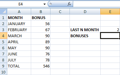

Step 2: Type the formula in the cell E4 as =SUM (OFFSET (B1, COUNT (B: B)-E 3+1, 0, E 3,1)).

Step 3: Press Enter. The sum of the bonus value for the last two months is displayed in cell E4.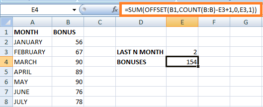

The above worksheet will display the result as 154, the sum of values of the last two months.

The formula explanation is as follows,

Reference- In the formula, B1 acts as a header which the values present in the column need to sum.

Rows- To calculate the cells in column B, the COUNT or COUNTA function is used. The difference between COUNT and COUNTA is the COUNT function returns the number of cells containing value where the last 'N'months is subtracted, and value 1 is added. COUNTA function returns all the cells in the column. Hence 1 is not added.

Columns - The number of columns to offset is zero.

Height- The value 'E3' describes the number of rows to be summed as mentioned in E3.

Width- Here, the width is mentioned as 1.

Example 2.2 - How to calculate the Average for the data using the OFFSET function?

To calculate the Average for the selected data, the steps to be followed are,

Step 1: Enter the data in the worksheet as follows,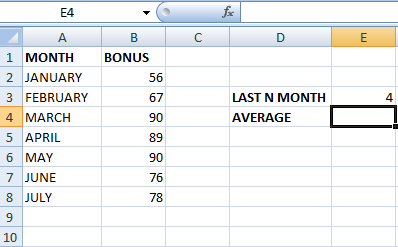

Step 2: Here, to calculate the Average for 'N' months, type the formula in the cell E4 as =AVERAGE (OFFSET ($B$1, COUNT (B: B)-$E$3+1, 0, $E$3, 1)).

Step 3: Press Enter. The Average for the selected month will display in cell E4.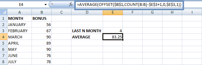

The above worksheet will display the result in cell E4, which is the Average for April, May, June, and July.

Example 2.3 - How to calculate the Maximum Value for the data using the OFFSET function?

To calculate the maximum value for the selected data, the steps to be followed are,

Step 1: Enter the data in the worksheet as follows,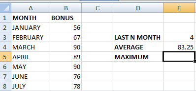

Step 2: To find the maximum value in the given data, type the formula in the cell E5 as =MAX (OFFSET (B1, COUNT (B: B)-$E$3+1, 0, $E$3, 1)). Here the maximum value for April, May, Jun, and July month is calculated.

Step 3: Press Enter. Among the four months, the maximum value is displayed in cell E5.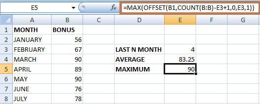

Here the result is displayed as 90, which is the maximum value among the data from April-89, May 90, June-76, and July 78.

Example 2.4- How to calculate the Minimum Value for the data using the OFFSET function?

To calculate the minimum value for the selected data, the steps to be followed are,

Step 1: Enter the data in the worksheet as follows,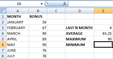

Step 2: To find the minimum value in the given data, type the formula in the cell E5 as =MIN (OFFSET (B1, COUNT (B: B)-$E$3+1, 0, $E$3, 1)). Here the minimum value for April, May, Jun, and July month is calculated.

Step 3: Press Enter. Among the four months, the minimum value is displayed in cell E5.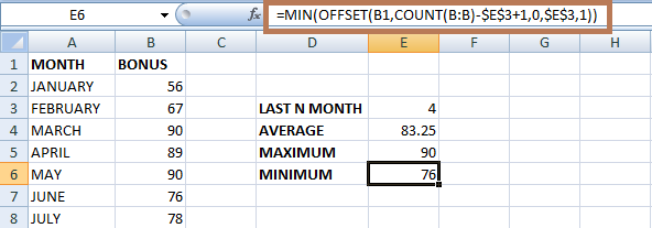

Here the result is displayed as 76, which is the minimum value among the data from April 89, May 90, June 76, and July 78.

From examples 2. 2, 2.3, and 2.4, the advantage of using the OFFSET function in MAX, MIN, and AVERAGE functions is every time, the user needs not have to modify the formula when the source table is edited. It calculates the last four data by default when new rows are added or deleted in the worksheet.

Excel offset in VLOOKUP and HLOOKUP.

As the name suggests, VLOOKUP and HLOOKUP are called Vertical lookup and Horizontal lookup. The vertical lookup returns the value present to the right of the lookup column. The horizontal lookup returns the value present to the left of the lookup column.

VLOOKUP

An example of the VLOOUP function is as follows,

Example 3: The given data shows the month and bonus. Retrieve the data for a specified month using the VLOOKUP function.

Step 1: Enter the data in the worksheet as follows,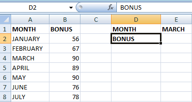

Step 2: Select the cell E2, where the user wants to display the result, and type the formula as =VLOOKUP (E1, A2:B8, 2, FALSE)

Step 3: Press Enter. The VLOOKUP function returns the value to the right of the lookup column.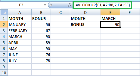

The above worksheet will display the result as 90, the present value right towards the specified data MARCH.

What happens if the data is swapped?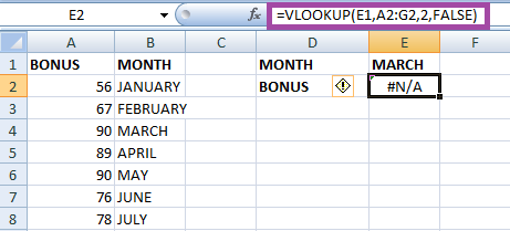

The above worksheet will display the result as not applicable as the data is swapped because the VLOOKUP returns the value only to the right of the lookup column.

Example 4: How to calculate the upper lookup in Excel?

From example 3, the VLOOKUP calculates the data present on the right. The steps to return data which is present upper ward is as follows,

Step 1: Enter the data in the worksheet as follows,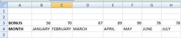

Step 2: Select a new cell and type the formula as =OFFSET(B3:H4,0, MATCH(B1, OFFSET(B3:H4,1,0,1, COLUMNS(B3:H4)),0)-1,1,1).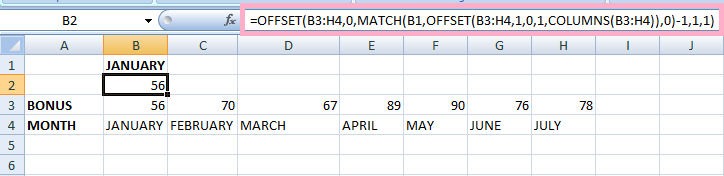

The above worksheet will display the result as 56, the value of the specified month of January.

HOOKUP

The HLOOKUP function is called a sibling of VLOOKUP. It looks for a value at the top of the row of a table or array of values and returns the same value in a similar column where the user specified the row.

Syntax

Lookup_value - It refers to the value to be searched in the table's top row. The value is either a text string or a reference.

table_array is a reference or range of array where the specified data is searched or looked up.

Row_index_num - The row index number is present in the array table where the matching value is returned.

For example, if the row index number is 1, it returns the value from the topmost row in the table array, and if the row index number is 2, it returns the value from the second row of the table array.

Range_lookup - The range lookup function accepts a Boolean value. The boolean value is used to indicate an approximate match or exact match. Here TRUE indicates an approximate match, and FALSE indicates an exact match.

An example of HLOOKUP is as follows,

Example 5: Retrieve the specified data from the table using the HLOOKUP function.

Step 1: Enter the data in the worksheet, which contains the mark of students of various subjects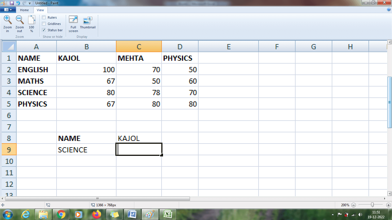

Step 2: To find the Science Mark of Kajol, enter the formula in the cell C9 as follows, =HLOOKUP ("KAJOL", A1:D5, 4, FALSE).

Step 3: Press Enter. The HLOOKUP function retrieves the science mark of Kajol from the given data.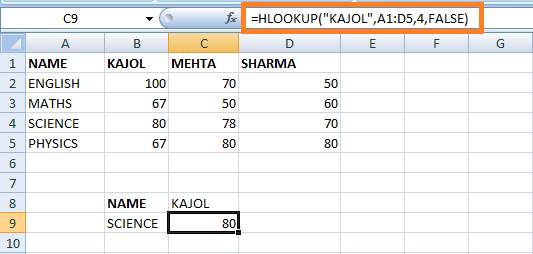

The formula "KAJOL" is called the lookup value, and A1:D5 is the table array. 4 is the row index number where the HLOOKUP value fetches the data from the fourth row, and FALSE indicates the exact match.

Example 5.1: Retrieve the Physics mark of the student who got 100 marks in English.

The steps to be followed are,

Step 1: Enter the data in the worksheet, which contains the mark of students of various subjects

Step 2: Select a new cell where the user wants to display the result and enter the formula as= HLOOKUP (100, B2:D5, 4, FALSE)

Step 3: The result will be displayed as 67, where the student who got 100 marks in English.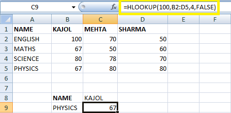

From the above formula, 100 is called the lookup_value of a student who got 67 in Physics. B2:D5 is the given date range, and 4 is the row index number where the HLOOKUP function returns the value. False is called range lookup, and only the exact match is needed.

Example 5.2: Retrieve the Maths Mark of a student whose name starts with 'S'.

Using the same table in example 5.1, the steps to be followed are,

Step 1: Enter the data in the required worksheet

Step 2: To find the Math Mark of a student starting with 'S', select a new cell and type the formula as = HLOOKUP ("S*", A1:D5, 3, FALSE).

Step 3: Press Enter. The result will be displayed in the selected cell, the Math Mark of Sharma.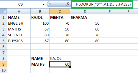

The above worksheet will display the result as 60, which is the Math Mark of Sharma, whose name starts with 'S'.

In the formula, the letter 'S*' is called LOOKUP value where the name starts with S. Table range or array is A1; D5. Three indicate the row index number. FALSE describes the exact match.

Example 5.3: Retrieve the specified data from two tables using the HLOOKUP function.

To retrieve the data from two tables, the steps should be followed are,

Step 1: Enter the data in the worksheet as shown below,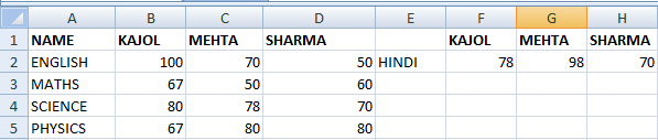

Step 2: To find the HINDI mark of the student, enter the formula in the cell =HLOOKUP (B1, $F$1:$H$2, 2, FALSE)

Step 3: The result will be displayed as 78, which is the Hindi mark of Kajol.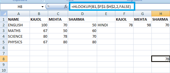

The above worksheet will display the result as 78, which is the Hindi Mark of Kajol. Using Fill Handle, the data are entered in row 6. As usual, in the formula, the B1 is called the lookup value, $F$1:$H$2 is called the cell range or array range, 2 indicates the row index number, and FALSE indicates the exact match in the table.

Example 5.4: From the given data, find the melting point of Hydrogen using the HLOOKUP Function.

To find the melting point of Hydrogen, the steps to be followed are,

Step 1: Enter the data in the worksheet as follows,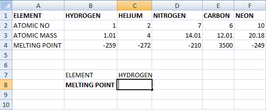

Step 2: Select a new cell, namely C7, and Enter the formula as = HLOOKUP (B1, A1:F4, 4, FALSE).

Step 3: Press Enter. The HLOOKUP function returns the Melting point of Hydrogen in cell C7.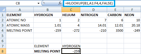

The melting point of Hydrogen is - 259, which is displayed in cell C7. The formula B1 is called HLOOKUP, A1:F4 is called cell range or table array.4 is called row index number. FALSE denotes the exact data match of the table.

Example 5.5: Find the Melting point of the element whose Atomic mass is less than or equal to 2.

To find the specified data, the steps to be followed are,

Step 1: Here, the data is similar to the data in Example 5.4.

Step 2: Select a new cell and enter the formula as =HLOOKUP (2, B3:F3, 2, TRUE).

Step 3: Press Enter. The result will be displayed in the selected cell, the melting point of data whose atomic mass is less than or equal to 2.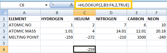

The melting point of Hydrogen is present in the selected cell. From the formula, 2 is the lookup value, and B3:F4 is the table range or array .2 indicates the row index number. TRUE indicates the appropriate value.

Summary

The above tutorial explains the various functions and formulas of creating a dynamic named range in Excel.