Extracting numbers from the string

How to extract numbers from the string?

By default, excel consists of various functions and formulas for retrieving the specified or selective data based on the requirement. The data entered by the user is text, numbers, or a combination of both. Sometimes there is a need to extract or parse the data for calculation purposes. If the data length is short, the user can retrieve the data manually. Even though the manual process works, it takes more time and sometimes leads to errors, which is impossible in large data sets. To rectify this issue, Excel provides the necessary formulas and functions to extract the text or number from the text string. Different methods are available to extract the text from the text string. But a bunch of functions is nested together to extract numbers from a text string. Here in this tutorial the methods to extract the number from the text string are explained in this tutorial.

Example 1: Extract the numbers present at the data's beginning using the formula.

To extract the numbers which are present at the beginning of the data, the steps to be followed are,

Step 1: Enter the data in the worksheet, namely A2:A6

Step 2: Select a new cell where the user wants to display the result and enter the formula as = SUBSTITUTE(A2, RIGHT(A2, LEN(A2)-MAX(IFERROR(FIND({0,1,2,3,4,5,6,7,8,9}, A2)," ))),"")

Step 3: Press Enter. The result will be displayed in the selected cell. To display the result for all cells, drag the formula toward cell B6.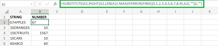

The above worksheet parses the numbers from the text string, which is displayed in cell A2:A6.

The formula explanation is described as follows,

Here from the above data, it is a combination of text and alphabets. Hence various functions are nested together, such as MAX, RIGHT, and LEN.

MAX returns the largest value in the function

RIGHT extracts the specified number of characters from the right side of the string

LEN is used to find the length of the given string

The functions mentioned above are used to find the number's position and remove the text from the string.

For a detailed description, the formula is breakdown as follows,

FIND({0,1,2,3,4,5,6,7,8,9},A2)

The FIND function finds the position of all numbers present in cell A2. It returns the #VALUE! Error except the numbers six and seven because it can't be able to locate the other numbers such as (0, 1, 2, 3, 4, 5, 8, 9). Hence it returns the position of 6 and 7 as one and two in cell A2, respectively.

IFERROR(FIND({0,1,2,3,4,5,6,7,8,9},A2),"")

The IFERROR function's purpose is to make all the error elements present in the array blank and return the array formula.

MAX(IFERROR(FIND({0,1,2,3,4,5,6,7,8,9},A2)

The MAX function finds the highest value present in the array element.

LEN(A2)-MAX(IFERROR(FIND({0,1,2,3,4,5,6,7,8,9},A2)

The LEN function extracts or removes all text characters from the cell. So first, the length of the string is calculated and subtracted from the position of the numeric value. Here 7-2=5.

RIGHT(A2,LEN(A2)-MAX(IFERROR(FIND({0,1,2,3,4,5,6,7,8,9},A2)

Here RIGHT function is used to extract the five characters to the right of numeric values, which is from the 2^nd character.

Applying the SUBSTITUTE function removes this string and replaces it with a blank cell. Hence the result will be displayed as "APPLE". Finally, the numeric value will be displayed as a result as 67.

The working process of the formula is shown below,

SUBSTITUTE(A2,RIGHT(A2,LEN(A2)-MAX(IFERROR({#VALUE!,#VALUE!,1,#VALUE!,#VALUE!,2,#VALUE!,#VALUE!,#VALUE!,#VALUE!}

),""))),"")
=SUBSTITUTE (A2, RIGHT (A2, LEN (A2)-MAX ({","", 1,","", 2,",","","}<
)),"")
=SUBSTITUTE (A7, RIGHT (A2, LEN (A2)-2),"")
=SUBSTITUTE (A7, RIGHT (A7, 7-2),"")
=SUBSTITUTE (A7,"APPLE","")
=67

Example 2: How to extract numbers from the text if it is present anywhere in the data?

To extract the text which is present anywhere in the data, the steps to be followed are,

Step 1: Enter the data in the worksheet, namely A1:A6.

Step 2: Select a new cell where the user wants to display the result and type the formula as =TEXTJOIN(", TRUE, IFERROR(MID(A2, ROW(INDIRECT("1:"&LEN(A2))),1)*1,")).

Step 3: Press Enter. The nested functions extract the numbers which are present anywhere in the data. To display the data for the remaining cell, drag the formula toward cell B6.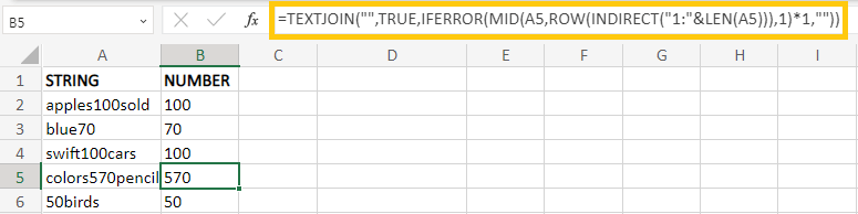

From the worksheet shown above, the nested function parses the numbers from the text string and displays the result in the selected cell.

The explanation of the formula is described as follows,

INDIRECT- This function returns the reference to the range of values

ROW- It returns the row number of a reference.

MID - It extracts the mentioned number of characters from the string

TEXTJOIN - This function combines the text from the strings or range using a delimiter.

LEN (A2) - It returns the string length present in cell A2.

(INDIRECT ("1:"&LEN (A2)))- It returns the reference to the row from 1 to 12

ROW (INDIRECT ("1:"&LEN (A2))), 1) - This function returns the row number for the specified row. Hence the ROW function returns the array as {1; 2; 3;4;5;6;7;8;9;10;11;12;13}

(MID (A2, ROW (INDIRECT ("1:"&LEN (A2))), 1) - The MID function is used to extract the character present in A2 and returns the array in the format of separate elements such as {"a"; "p"; "p"; "l"; "e"; "s"; "1"; "0"; "0"; "s"; "o"; "l"; "d"}

IFERROR (MID (A2, ROW (INDIRECT ("1:"&LEN (A2))), 1)

The IFERROR function replaces all the characters with non-numeric ones. It multiplies all characters with 1. If the element present is non-numeric, it returns an error. If it is a numeric value, it returns the same value, which is multiplied by one. The result will be displayed as,

{"";"";"";"";"";""; "1"; "0": "0":"":"":"":""}

=TEXTJOIN("",TRUE,IFERROR(MID(A2,ROW(INDIRECT("1:"&LEN(A2))),1)*1,""))

The TEXTJOIN function combines the remaining elements which are present. Here the numeric values are only present. Therefore, it combines the numeric values as 100.

The formula works in a nutshell as follows,

=TEXTJOIN (", TRUE, IFERROR (MID (A2, ROW (INDIRECT ("1:"&13)), 1)*1,"))

=TEXTJOIN("",TRUE,IFERROR(MID(A2,{1;2;3;4;5;6;7;8;9;10;11;12;13},1)*1,""))

=TEXTJOIN("",TRUE,IFERROR({"a";"p";"p";"l";"e";"s";"1?;"0?;"0?;"s";"o";"l";"d"}

*1,""))

=TEXTJOIN("",TRUE,IFERROR(MID(A2,{1;2;3;4;5;6;7;8;9;10;11;12;13},1)*1,""))

=TEXTJOIN ("", TRUE, {"";"";"";"";"";""; 1; 0; 0 ;"";"";"";""})

=100

Example 3: How to extract numbers from the text if it is at the end of the data?

To extract the text which is present at the end of the data, the steps to be followed are,

Step 1: Enter the data in the worksheet, namely A1:A6.

Step 2: Select a new cell where the user wants to display the result and type the formula as =SUBSTITUTE(A2, LEFT(A2, MIN(IFERROR(FIND({0,1,2,3,4,5,6,7,8,9}, A2),"))-1),"")

Step 3: Press Enter. The nested functions extract the numbers present at the data's end. To display the data for the remaining cell, drag the formula toward cell B6.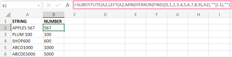

From the worksheet shown above, the nested function parses the numbers from the text string and displays the result in the selected cell. The formula explanation is as follows,

FIND({0,1,2,3,4,5,6,7,8,9}, A2)- The FIND function is used to find the positions of the given numbers in cell A2. It displays the result as,

{#VALUE!,#VALUE!,#VALUE!,#VALUE!,#VALUE!,#VALUE!,5,6,7, #VALUE!}

It returns the error message except for the position 7^th, 8th, and 9th digits. The FIND functions won't be able to find the numbers except 5, 6, and 7 in cell A2. Hence the 7^th, 8^th, and 9^th positions return the value as 5, 6, and 7.

IFERROR(FIND({0,1,2,3,4,5,6,7,8,9},A2)

The function of IFERROR is to return all the error elements present in the array with blank cells except the numeric value. Hence the array will look like this,

{"","","","","","","", 5, 6, 7,""}

MIN(IFERROR(FIND({0,1,2,3,4,5,6,7,8,9},A2)

The function of the MIN element is to return the element present in the array with the least value. The position of the first numeric value is displayed. Here in this example, the position of the first numeric value is 7.

LEFT(A2,MIN(IFERROR(FIND({0,1,2,3,4,5,6,7,8,9},A2) ,""))-1),"")

Here the LEFT function extracts all the text characters in the data. It is extracted from backward, which means the MIN function returns the value as 7, which is the starting position of the numeric value. The value 1 is subtracted from 7(7-1=6). The result will be obtained as "APPLES".

=SUBSTITUTE(A2,LEFT(A2,MIN(IFERROR(FIND({0,1,2,3,4,5,6,7,8,9},A2) ,""))-1),"")

The SUBSTITUTE function replaces the obtained text string (APPLES) with blank. Hence the result obtained is 100.

The working process of the formula is shown below as follows,

=SUBSTITUTE(A2,LEFT(A2,MIN(IFERROR(FIND({0,1,2,3,4,5,6,7,8,9},A2),""))-1),"")

=SUBSTITUTE(A2,LEFT(A2,MIN(IFERROR({{#VALUE!,#VALUE!,#VALUE!,#VALUE!,#VALUE!,#VALUE!,5,6,7,#VALUE!}),""))-1),"")

=SUBSTITUTE (A2, LEFT (A2, MIN ({",",",",","", 5, 6, 7,"}))-1),"")

=SUBSTITUTE (A2,"APPLES","")

=100

Example 4: How can a Flash Fill method extract numbers from the text string?

The Flash Fill method is one of the easiest methods to extract numbers from the text string. If it follows the pattern present in the first cell. The steps to be followed are,

Step 1: Enter the data in the worksheet, namely A1:A6

Step 2: Select a new cell where the user wants to display the result, B2. Type the numeric value in B2, present in the data A2. After entering the data, press CTRL+E or click Data>Flash Fill.

Step 3: Right-click cell B2 and drag toward B6. The flash fill method automatically fills the data.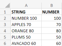

The above worksheet fills the data using the flash fill method.

Example 5: How to extract a five-digit number from the given Data?

The formula uses the Concatenation and Sequence function to get the five-digit text character from the string. The steps to be followed are,

Step 1: Enter the data in the worksheet, namely A1:A6

Step 2: Select a new cell where the user wants to display the result namely B2. Type the formula in the cell as =CONCAT (IFERROR (0+MID (A2, SEQUENCE (LEN (A2)), 1),")).

Step 3: Press Enter. The result will be displayed in the selected cell.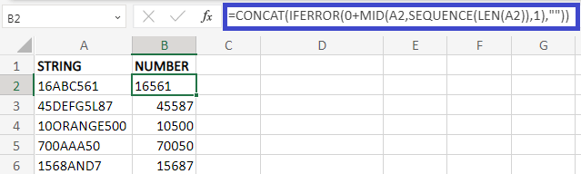

The formula explanation is as follows,

(LEN (A2))- The length function returns the string length present in cell A2. It returns the output as 8.

SEQUENCE (8) - The SEQUENCE function returns the Data's first eight positions. The output will be displayed as {1;2;3;4;5;6;7;8}

MID (A2, SEQUENCE (LEN (A2)), 1),")) - The output obtained as {"1"; "6"; "A"; "B"; "C"; "5"; "6"; "1"}. Add 0 to the string 0+{"1"; "6"; "A"; "B"; "C"; "5"; "6"; "1"}. The result will be displayed as {1; 6; # VALUE!; # VALUE!; # VALUE!;5;6;1}

(IFERROR (0+MID (A2, SEQUENCE (LEN (A2)), 1),""))- The IFERROR function replaces the error value with blank, and hence the output will be displayed as

{1; 6;"";"";""; 5; 6; 1}

CONCAT (IFERROR (0+MID (A2, SEQUENCE (LEN (A2)), 1),""))

The CONCATENATION function is used to add the numbers present in the output. Hence the result will be displayed as 16561.

Example 6: How to extract only numbers from the given Data using Excel VBA Macro?

Excel VBA Module helps to extract the numbers from the text string. It is one of the alternative methods for formulas and functions. The code asks the user to enter the input and output ranges where the user can enter the respective data range.

The steps to use Excel VBA Module is as follows,

Step 1: Press ALT+F11. A VBA window will open.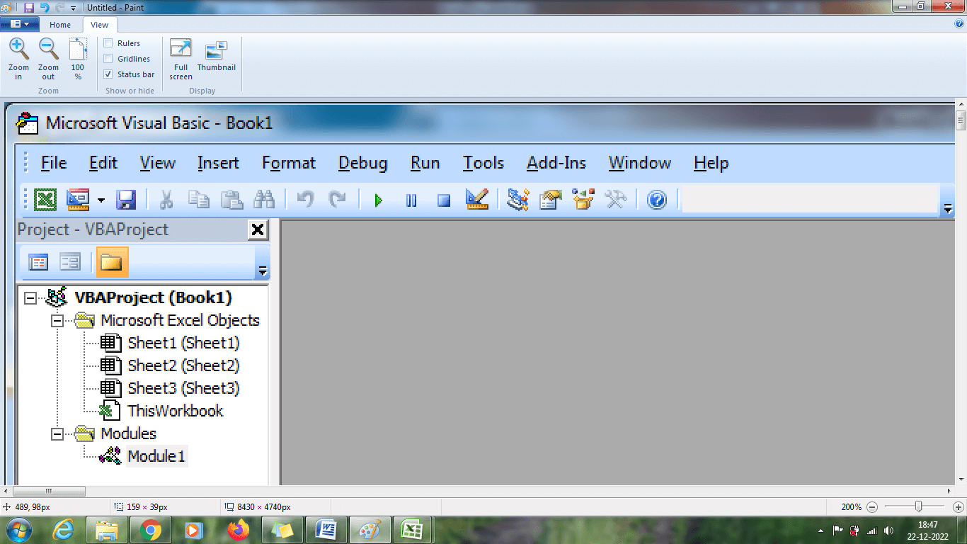

Step 2: Click Insert >Module command. A new module window will display.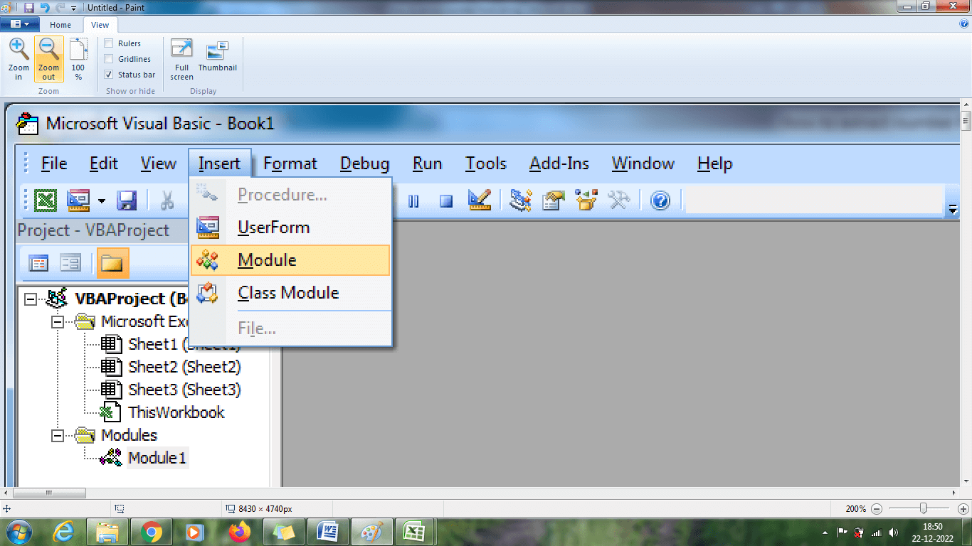

Step 3: Enter the code in the module window. The code is as follows,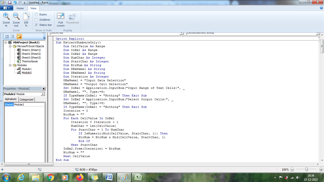

Step 4: To execute the code, press F5. An "Input Selection box "will appear.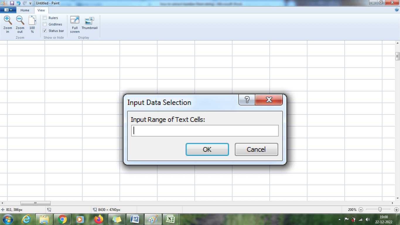

Step 5: Enter the specified row as $A$2:$A$6.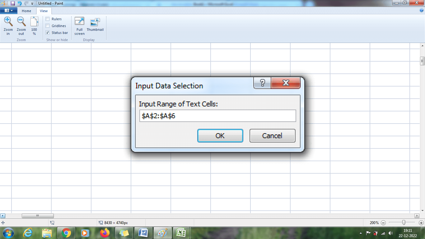

Step 6: An Output cell Selection box will display. In that, enter the specified output cell.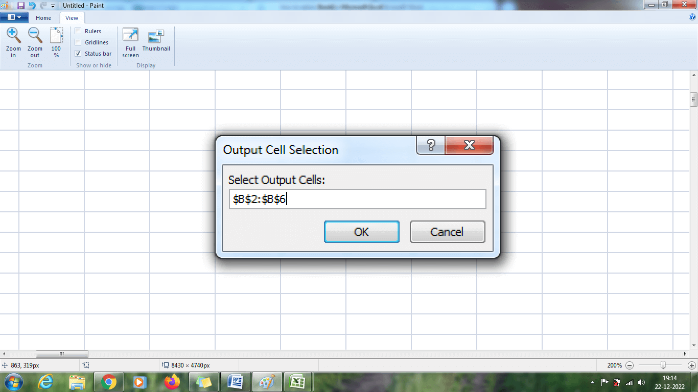

Step 7: After entering the data, click the output cell range B2:B6 and press Enter. The text numbers present in the data are parsed and displayed in the output column B2:B6.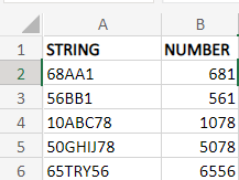

The above worksheet shows the result in cell B2:B6 which is the numbers parsed from the given data.

Example 7: Extract the numbers from the given Data using the delimiter function

One of the easiest alternative functions to parse the numbers from the given text is using a delimiter. The steps to be followed to apply the delimiter function are as follows,

Step 1: Enter the data in the worksheet, namely A1:A6. Here the Data is entered in the rows where there occurs a separation between text and numbers, as shown,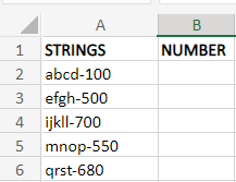

Step 2: Select the data from A1:A6.Click the Data>Text to columns option.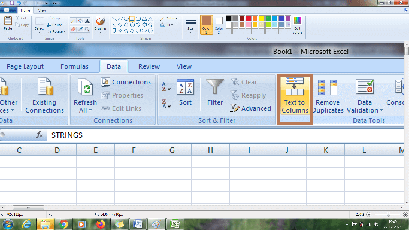

Step 3: Convert Text to Column Wizard will open. In that, choose the Delimiter option. Click Next.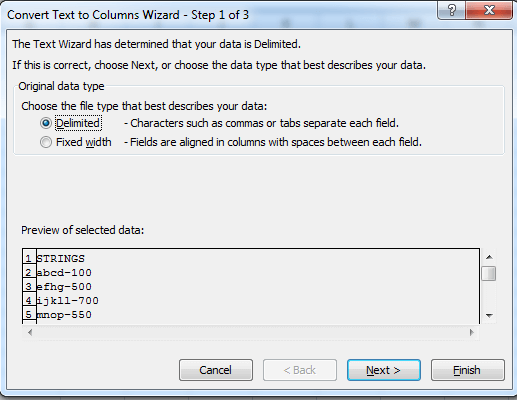

Step 4: Convert Text to Column Wizard dialogue box2 will open. Click the other option and type the '-' hyphen symbol in the box. Click Next. The data preview is shown in the dialog box. Click Finish.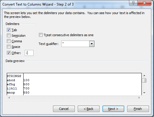

Step 5: The result will be displayed in cell B2:B6, where the numbers are extracted from the given data and displayed in the selected cell.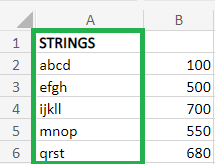

Using the delimiter function, the specified Data is extracted from the given Data, which is a quicker and easier process.

Summary

Methods including functions, formulas, delimiter, and Excel VBA methods are used to extract the numbers from the text. These functions and formulas work efficiently to extract the number from the text. The various methods to extract the numbers from the text are described in the examples. The methods and functions are clearly explained in this tutorial.

Next TopicFinding Top or Bottom 'N' values in Excel

← prev