Formula reference in Excel

Formulas are the significant and most used concept in Microsoft Excel worksheets. Though working with formula, the most important concept is cell reference. As easy as it seems, Formula reference confuses many Excel users. This tutorial will cover the definition of formula cell and range reference, types of cell references in Excel, steps to implement cell references, and many more!

What is a Formula reference?

Excel Formulas that you create mostly contain references to either cells or ranges. These references are important because they allow your formulas to operate dynamically with the data included in those cells or ranges. Let's understand the difference between a cell reference and a range reference.

A cell reference (also commonly known as cell address) is defined as an intersection of a column (typed in a letter) and a row (entered in a number) that specifies a particular cell in your Excel worksheet.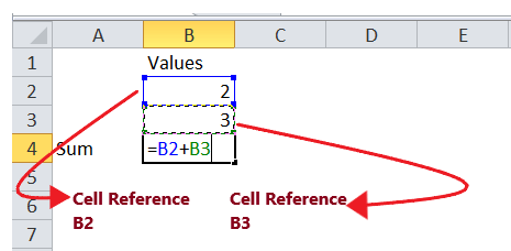

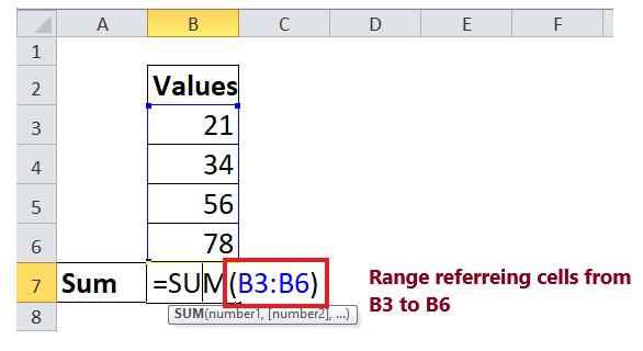
Example: The cell reference B2 refers to the cell at the intersection of column B and row 2; B3 refers as a combination of cell in column B and row 3, and so on.

Whereas,

A range reference is defined as the cell address of the upper-left cell and the lower right cell divided with a colon symbol.

Example: The cell range B3:B6 includes 4 cells from B1 through B6.

How to create a reference in Excel

To create a cell reference in your Excel worksheet, follow the below given steps:

1. Put your cursor on the cell where you want to enter your formula.
2. Start typing the formula using equal sign (=).
3. Do one of the following:
   • Enter the reference directly in the cell or in the formula bar, or
   • Select the cell you want to refer.
4. Enter the rest of the formula and press the Enter button to execute it.
5. For instance, in the below example, as you can see, we have two values in cells A1 and A2. Now, to add both the values, we will type = cell reference of B2 (B2), type the plus sign, cell reference of B3 (B3), and press Enter.

You will have the following output.

To create a range reference in your Excel worksheet, follow the below given steps:

1. Put your cursor on the cell where you want to enter your formula.
2. Start typing the formula using equal sign (=).
3. Do one of the following:
   • Enter the first cell reference from where you would like to start the reference
   • Put a colon (:) to separate the first and last cell
   • Mention the last cell at which you want the range reference to end.
4. Enter the rest of the formula and press the Enter button to execute it.
   For example, if you want to add up the values in cells B3, B4, B5, B6. One way is to write = SUM (B3 + B4 + B5 + B6). But this is a lengthy method. The same formula can be covered quickly using the range concept. Type the equal symbol (=) followed by the Excel SUM function, refer to the cells from B3:B6, and press the Enter button.
   You will have the following output:
   
5. While working with Excel rows and columns, sometimes you may require to refer to the entire row or column. In such situations, directly click on the top of your row number or the column letter.
6. For example, if you wish to calculate the sum for all the cells present in row 2 Type the equal symbol (=) followed by the Excel SUM function, and then click on the top of your row 2 to include the row 2 reference in your formula. It will indicated by B:B.

Types of Formula reference

While using a cell (or range) reference in a formula, you can use three types of references - relative, absolute, and mixed references. When you are writing a formula for a single Excel cell, you can choose any reference type. But sometimes, we don't type the formula again, and instead, we copy and paste it to other cells. We must apply a suitable address type to incorporate this because relative and absolute cell references act differently when copied to other cells.

Relative Cell References

A relative reference is defined as the cell or range reference mentioned without the $ symbol in the row and column coordinates, such as B1 or B2:B12. By default, all cell references existing in Excel your Excel worksheet are relative.

When you copy the formula carrying data with relative cell references to different cells, the row, and column references also change because the references are offset from the current row and column. By default, Excel creates relative cell references in formulas.

When repositioned or copied across different Excel cells, relative references change based on the relative position of the current rows and columns. Sometimes, we want to repeat the same formula across different rows or columns, and we simply drag the formula to different cells. In those cases, you need to use relative cell references.

Let's suppose you have the given below formula in cell C3:

=B3*10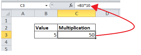

Next, when we copy the formula in cell C3 to another row in the same column. In the below image, we have copied it to cell C4, because we have used relation reference in cell C3, while copying the formula it will automatically adjust for row 4 (B4*10).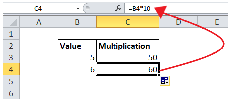

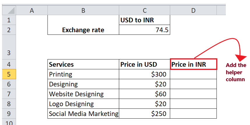
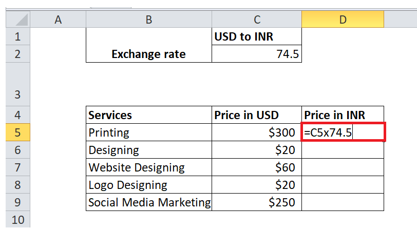
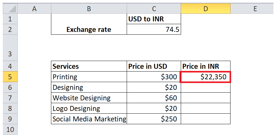
If you copy the same formula further down the Excel in the same column will keep changing the column reference accordingly and give you the output

If you copy the formula containing the relative cell reference to another row and column, you will notice that Excel will change both the row and column coordinates.

Relative cell references are the most commonly used cell references while working with Excel formulas. It is because it is very convenient and helps to easily perform the same calculations across the entire worksheet. To understand it better, let's discuss a real-life example that will be solver using relative reference.

Example using relative reference in Excel

Question: In the below column you are given USD prices for different products. You want to convert the prices to INR so you can pursue the further calculation and do the analysis. It is given that the USD - INR conversion rate is 74.45 at the moment. Using the Excel relative cell reference, convert the USD prices to INR.

To convert USD prices to EUR using Excel relative cell reference, follow the below given steps:

1. In the data as the USD prices are mentioned in column B. Add a helper column in Column C where we will enter the formula to convert USD to INR.
   
2. Start the formula with =cell reference x 74.45. Since the data in Cell C3, so our formula becomes = C3 x 74.45
   
3. Press the Enter key to calculate the formula, and Excel will immediately display the output in the first helper cell.
   
4. We know that by default, all the cell references are relative. Therefore we will copy the formula to further cell.
5. Select the cell where you have typed the formula. Take your mouse cursor towards the end of the rectangular box.
6. You will notice the cursor will change into a small thin black cross. Drag it down the column to auto-fill the Excel cells. You will have the following output.

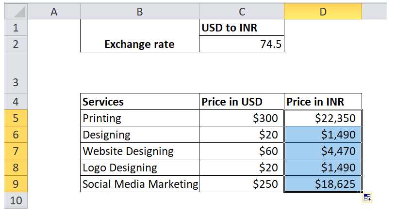
That's it! You will notice the relative cell reference formula is replicated to other cells where are cell values are automatically adjusted for each individual cell. To verify that a formula in each cell is calculated accurately, select any of the cells and look at the formula in the formula bar. For instance, here we have selected cell D7, and view that the cell reference in the formula is relative to row 7, exactly as it should be: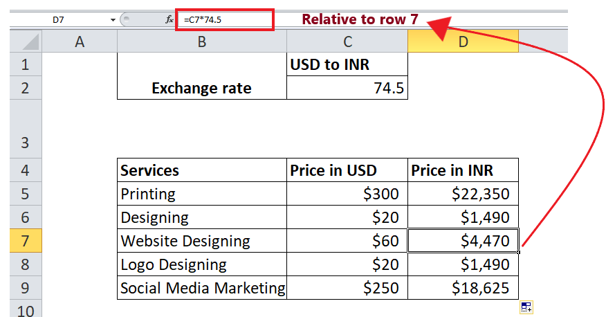

Absolute Cell References

"An absolute reference is defined as the cell or range reference that remains unaffected while copying the same formula to other cells. Absolute addresses are extremely helpful when you want to achieve multiple calculations with a value in a particular Excel cell or when you require to copy a formula to different cells without modifying references."

The advantage of using an absolute reference is that the row and column coordinates do not alter when you copy the formula because the reference is an actual cell address. To indicate an absolute cell reference, always use two dollar symbols before column coordinate and row coordinate.

For instance, absolute references $B$6 implies both the column and row coordinates are fixed.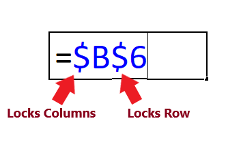

For example, if you want to add the additional marks (in cell C1) with the total marks obtained (given in column B). We will start the formula with equal sign (=),select the cell reference of marks field, and add the additional marks to it, where we will pass an absolute reference for cell C1. We will have the following formula

=B4*$C$1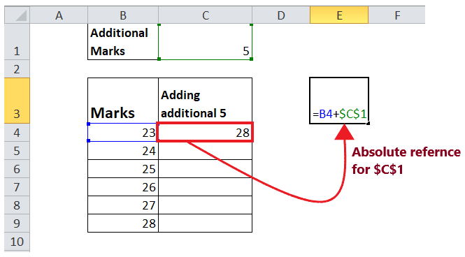

Copy the formula down column C by dragging the small thin black cross. The relative cell reference changes for all the cells, whereas the Absolute reference is constant across all the cells and will always be locked on the same cell ($C$1).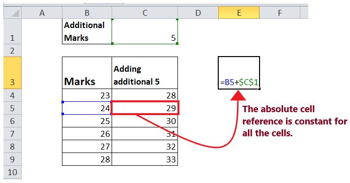

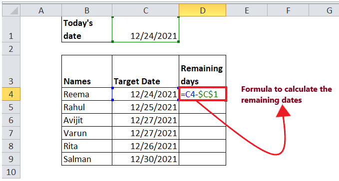
To understand it better, let's discuss a real-life example that can be easily solved using the concept of absolute cell reference.

Example using relative reference in Excel

Question: Calculate the remaining dates to achieve the sales target in a single formula using the concept of Relative and absolute cell references in Excel worksheet.

Calculating dates in Excel is one of the common use of absolute and relative cell references. Follow the below steps to calculate today's date in a single formula in Excel:

1. In the above example we have a list of Target sales dates in column C, and the current date in entered in cell C1. Add a helper column in Column D where we will enter the formula to convert find the remaining days to achieve the sales target.

2. You can calculate the number of days left by each account manager by using the following formula.

In the above formula, we have used a combination of relative cell reference and absolute cell reference. Each formula reference fulfills the given task:

• Relative reference for the cell carrying value of the target sales date (C4) because this cell reference will change when you copy the formula down the other row values.
• Absolute reference for the cell carrying today's date ($C$1) because this cell reference remains locked across the different cell.

3. Select the cell where you have typed the formula. Take your mouse cursor towards the end of the rectangular box. You will notice the cursor will change into a small thin black cross. Drag it over the cells you want to auto-fill.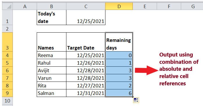

Mixed Cell References

"A mixed cell reference is defined as a cell or range reference in Excel wherein either the column or the row coordinate is fixed."

NOTE: To incorporate mixed reference press the F4 button.

Excel users often get confused between Excel absolute reference, and Excel missed reference and mistakenly uses both of them interchangeably. But both are different.

Excel absolute reference contains the dollar signs ($) with both the row and column. Therefore it freezes both the column and the row coordinate, whereas in the case of a mixed cell reference, at a time only a single coordinate is fixed (absolute) and the other (relative) will change based on a relative position of the row or column:

In other words, the Mixed cell reference is a combination of Absolute column and relative row. For instance, $A1 and A$1 are mixed references. But what is the difference between these two mixed references, since both contains cell A1?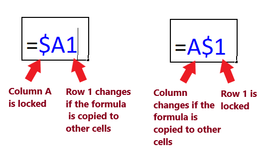

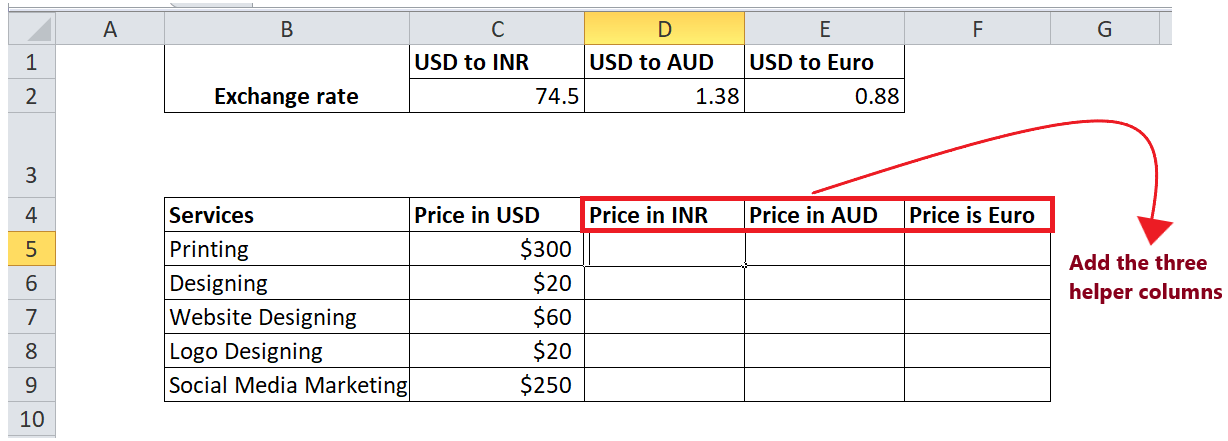
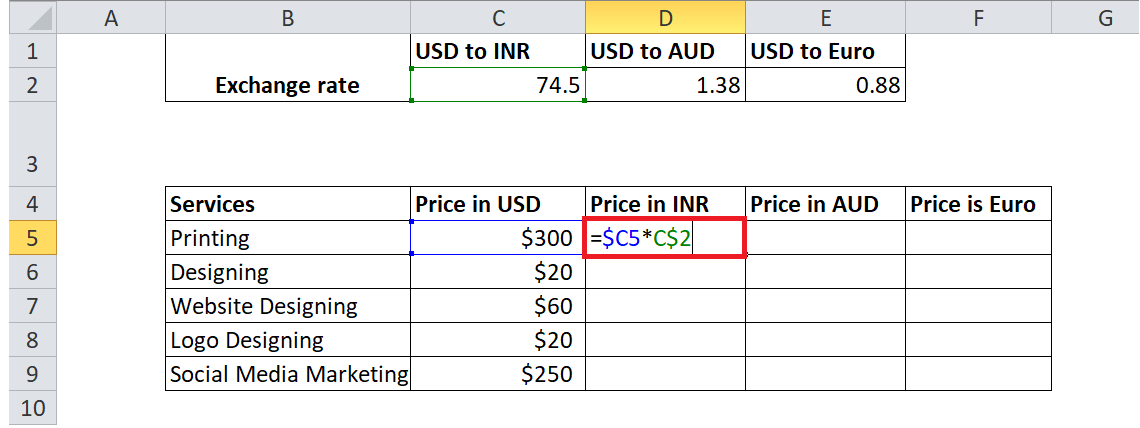
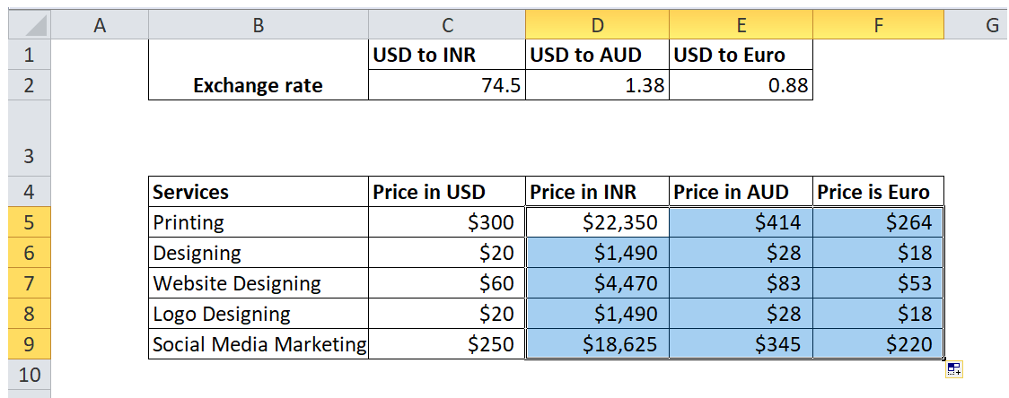
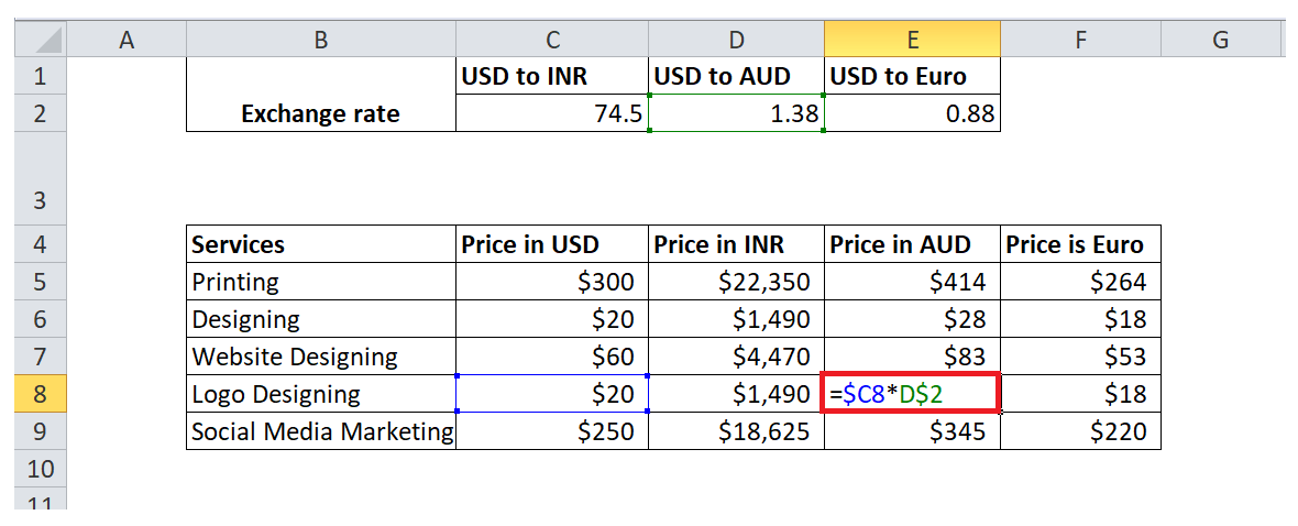
1. Absolute column letter and relative row number: $A1
   Column A is locked or absolute reference, the row is relative. If this formula is copied to other cells across the Excel worksheet, the $ sign in front of the column letter will be fixed to the specified column A so that it never changes. Without the dollar sign, the relative row reference changes depending on the row to which the formula is copied.
2. Relative column letter and absolute row number: A$1.
   Here column A is relative that changes according to the cell, and the row is relative. The row's reference is locked in this formula that won't change.

Formula Example using a mixed reference in Excel

Example 1: Using the currency conversion table, convert the dollar currency to different currencies with the help of only one single formula!

Since USD is the standard currency worldwide, we have taken the prices of services in USD. When dealing with international business, frequently you are asked to convert the prices. Let's enter the conversion rates in some row, say row 2, as shown in the screenshot below. Then follow the below steps to convert the USD currency to another:

1. In the above example, we have to convert the USD prices to different currencies. We will add three helper columns in Column D (Price in INR), Column E (Price in AUD), and Column F (Price in EURO), respectively.
   
2. You can convert USD to other currencies by using the following formula.
   =$C5*C$2
   
3. Select the cell where you have typed the formula. Take your mouse cursor towards the end of the rectangular box. You will notice the cursor will change into a small thin black cross. Drag it over the cells you want to auto-fill.
   
4. As you can see in the above screenshot, we have the output for 3 different price columns that we have calculated using the mixed cell reference type. Since we have dragged the formula, let' verify it once. Select any random cell from the output table, and cross-check the formula in the formula bar.
   For instance, let's select cell E8 (in the Price in the AUD Helper column). The formula that is displayed in its formula bar is =$C8*D$2 that takes a USD rate from cell C8 and multiplies it by the AUD conversion value in cell D2. Eureka! It is all correct and in the same orientation which we wanted.
   

The above formula was easy, but most of you might have been confused and thought about how exactly Excel knows which price value to take and which exchange rate to multiply it by. Yes, you guessed it right. It is all because of the mixed cell references. Let' understand the implementation of the above-used formula (=$C5*C$2):

• $C5 - It represents absolute column letter and relative row number. The dollar symbol is only added in front of the column to lock it, therefore Excel always uses the USD prices for all price conversions. In this formula the row reference is relative (used without dollar symbol) because you want to calculate the prices for each row individually. If it is copied to other cells across the Excel worksheet, the $ sign in front of the column letter will be fixed to the specified column A so that it never changes. Without the dollar sign, the relative row reference changes depending on the row to which the formula is copied.
• C$2 - It represents relative column letter and absolute row number. In this formula, all the exchange rates re mentioned in row 2, therefore we have locked the row coordinate by adding the dollar symbol next to the row number If it is copied to other cells across the Excel worksheet, no matter what the $ sign in front of the row number will be fixed to the specified row 2 so that it never changes. Without the dollar sign, the relative row reference changes depending on the column to which the formula is copied.

Switch between Formula cell references (absolute, relative, and mixed)

Microsoft Excel provides different ways of doing the same thing. While working with the formula, you can manually type the $ and implement various cell references or convert a relative reference to absolute or absolute to mixed. But the shortest and easiest way to incorporate the $ sign is by using the F4 key. Though it will speed things up for you, but there is a condition for the F4 shortcut to work, i.e., it is mandatory to have it in formula edit mode:

1. Select the cell that contains your formula.
2. Double click on the cell to enable the formula Edit mode. You can also press the F2 shortcut key to enable it.
3. Select the cell reference that you wish to change. For instance, we have selected cell reference A3.
4. Next, press the F4 key to switch the $ sign between four cell reference types.
5. We have selected a relative cell reference (A3) that contains no dollar ($) symbol, continuously hit the F4 key to switch between an absolute reference (with 2 dollar symbols on row and column respectively unlike $A$3), mixed absolute row (A$3), mixed absolute column ($A3), and then it will take you back to the original relative reference A3.