| |

Freeze Columns in Microsoft ExcelThe respective MS Excel or Microsoft Excel is powerful spreadsheet software that helps users record a huge amount of financial data. An Excel workbook consists of the several worksheets where each sheet can store many data records within multiple cells. When working with large sets of data within an Excel worksheet, it often becomes difficult to track, remember or compare the information. When we work around common data sets around the sheet and navigate to the right side of the worksheet, we may not see the corresponding headings. This is where freeze columns can be helpful as well. 
And in this particular tutorial, we will be learning the various step-by-step methods that will help us to lock or freeze out the columns in Microsoft Excel. We can quickly implement these methods using Microsoft Excel 2010; however, they can be used similarly in other versions of MS Excel. Before we move on to the methods, let us first briefly discuss using the Freeze Columns feature and how it can help us increase the readability of our Microsoft Excel worksheets as well. What is the Freeze Columns feature in Microsoft Excel?And the Freezing Microsoft Excel column is one of the valuable features to increase the readability and productivity of the data within a worksheet. It primarily helps compare or read data from the different parts of the sheet with easy navigation. Freezing an Excel column typically locks or freezes the position of the column so that it doesn't scroll through the database while navigating the sheet. When a column freezes, it locks its place while navigation through the other columns usually works.
Important Note: When we freeze one or more columns within the worksheet, they remain visible or fixed only for horizontal movements. If we scroll or navigate the worksheet downwards, the column values will also move vertically for the corresponding rows.How to freeze columns in Microsoft Excel?When working with large sets of data, there may be cases when we may need to freeze columns as well. Usually, we may need to freeze either one column or more than one column in a sequence. Fortunately, we can quickly freeze single or multiple columns in Microsoft Excel without limiting the number of columns to be frozen. Because of this, Microsoft Excel gives a more productive presentation, allowing us to read or compare data within a worksheet easily. Let us now discuss both the use cases where we may need to freeze a column in Microsoft Excel, including all the steps for freezing columns: Freeze a Single (side-Left) Column in Microsoft Excel.It is well known that Microsoft Excel allows us to freeze a single column in an entire sheet as well, and depending upon the requirement, we can easily choose to freeze the column from the beginning or middle of the sheet as well. When we need to freeze a column, Microsoft Excel gives the option to freeze only the first column. The first column does not refer to the first column of the worksheet. Instead, it targets or refers to the first column that appears as the first column (side-left column) in the active or visible area of the Excel window on the screen.
Step 1: First of all, we all must scroll down the worksheet to the right so that the column we want to freeze becomes the first column in the active or visible area of the Microsoft Excel window. In our example, we place column B as the first column or side-left column in the view area, as depicted below: 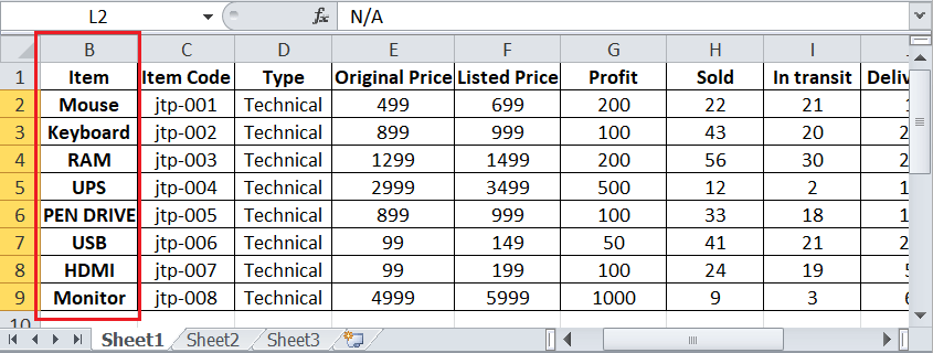
Step 2: Nextly, we are required to go to the View tab, and then we need to click on the drop-down button next to the Freeze Panes button, which is present just under the "Window section." Here, we have to click on the option that is none other than the 'Freeze First Column' respectively. 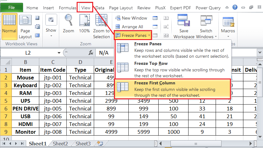
Step 3: After this, we are required to click on the 'Freeze First Column' option, then the respective column easily gets fixed immediately, which means that even if we navigate the sheet to the very right of the respective worksheet, the fixed column will not be scrolled. However, all other columns will scroll as usual.
Now in the above worksheet, we can easily see that column B is still visible on the far left side of the Microsoft Excel window even after navigating to the right side of the sheet. And it is essential to note that columns before Locked/Fixed/Frozen columns may not be visible. As in our example, column A is not visible. Freeze Set of Columns in Microsoft ExcelMicrosoft Excel also provides the option to freeze more than one column within a worksheet. However, some of the limitations are associated with this as well. We cannot freeze non-contiguous (non-adjacent) columns. If we want to freeze multiple columns, they must be sequenced. Also, Microsoft Excel does not offer the flexibility of freezing columns from the middle of worksheets. This means we cannot freeze any random set of columns in the middle of the sheet. Instead, we need to freeze all the columns exiting between the desired column and the first column of the worksheet.
Now in order to freeze a set of columns or multiple columns (i.e., from column A to E), we can perform the following steps respectively: Step 1: First, we must select the respective column right next to the desired set of columns we want to freeze. If we want to freeze columns A to E, we have to select the whole column F. To select the entire column, we can easily click on the column header from the leftmost area of the worksheet. Alternatively, we can select the first cell of the column (F1) respectively. 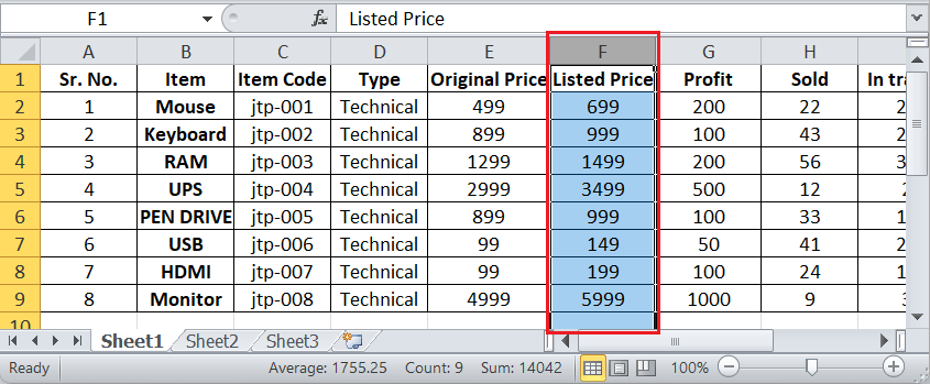
And if we only want to display columns B to E, we can quickly scroll a sheet to the right and place column B as the first column in the visible area on the screen. Step 2: Just after that, we select the column followed by the desired column set, and we are required to navigate to the View tab on the ribbon, and then we need to click on the drop-down arrow next to the Freeze Panes. Afterward, we need to select the 'Freeze Panes' option from the given list, as depicted in the following image: 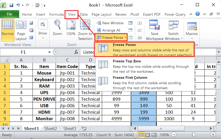
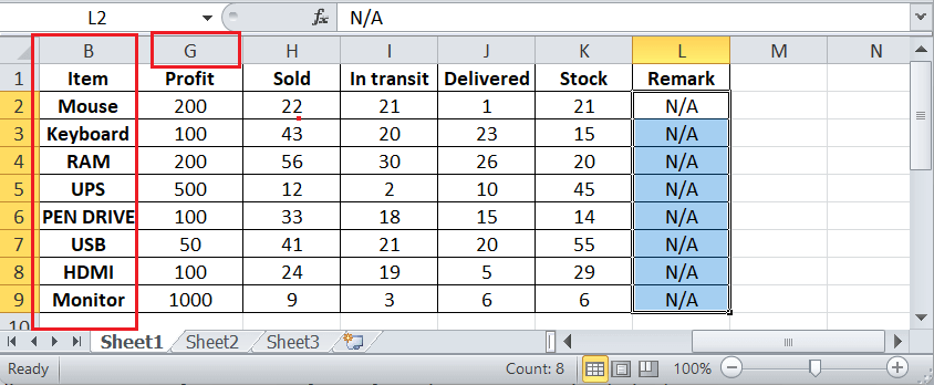
Step 3: Just after that, we need to click on the "Freeze Panes" option from the drop-down list; we will see a bold border (Grey Line) line exiting between columns E and F. This bold line indicates that the columns before this line are locked/fixed/frozen. 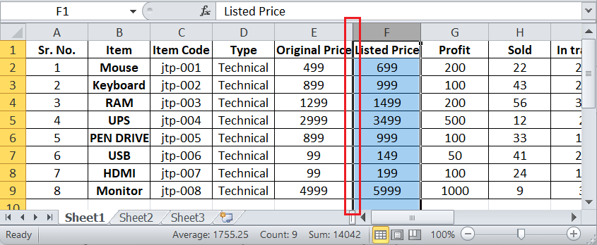
If we scroll down the sheet to the right, we will see that columns from A to E are still visible at the far left of the Microsoft Excel window. However, the other columns starting with column F are usually scrolling. 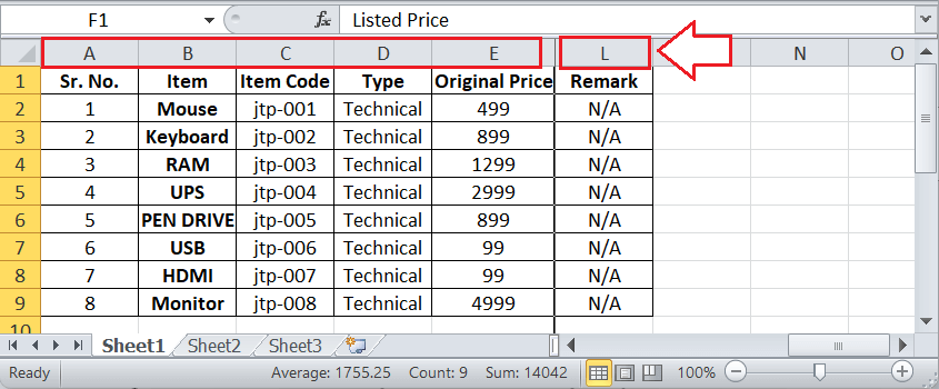
In the above example sheet, we can see that even after scrolling the sheet to column L, the initial five columns (columns A to E) are fixed to the far left of the Microsoft Excel window. Unfreezing an Excel Column or Multiple ColumnsThere may be cases when we have frozen the wrong columns or we no longer need frozen columns in the worksheet respectively. In such cases, unfreezing one or more columns in an Excel worksheet is straightforward. We can follow the below steps and unfreeze the locked column in one go: Step 1: First, we must select or display the specific worksheet where we want to unfreeze columns. Step 2: Nextly, we need to go to the 'View' tab, and then we are required to click on the 'Freeze Panes' drop-down arrow, and then we need to select the 'Unfreeze Panes' option. This will unfreeze or unlock all the columns in the selected sheet respectively. 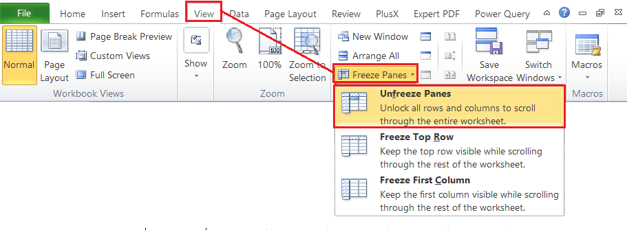
What are the essential points to Remember about the Freezing of the Columns in Microsoft Excel?The various essential points that need to be remembered by an individual about the freezing of the columns in Microsoft Excel are as follows:
Next TopicFreeze Rows in Excel
|
 For Videos Join Our Youtube Channel: Join Now
Feedback
- Send your Feedback to [email protected]
Help Others, Please Share


