Get Pivot Data Function in Microsoft Excel

The word GETPIVOTDATA means getting all the respective Data from the Pivot Table. And it is termed to be the specific kind of pivot table lookup function that is present under the Lookup and Reference function.

This particular function primarily helps in the extraction of a specific amount of data from specified fields in a Pivot Table. The Pivot Table is usually an analysis tool that, in turn, is used to efficiently summarize a vast amount of data in a readable manner.

Furthermore, these particular Getpivotdata function can query out the pivot table and then after that can retrieve the specific data which are primarily depending upon the table structure instead of the references effectively.

GETPIVOTDATA Formula in Microsoft Excel

The Formula used for the GETPIVOTDATA Function in Microsoft Excel is seen in the figure below.

And the above function consists of the following parameters that are as given below:

1. Data Field.
2. Pivot Table.
3. [Field1, Item1], [Field2, Item2], [Field3, Item3].

And now, before explaining the syntax of the "GETPIVOTDATA" Function one by one, let us first see a simple example.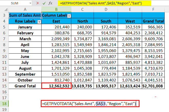

We are then looking for the Grand Total Amount of the particular Region East from the above mentioned function.

1. Data Field: As from the above example, the particular data field primarily means the heading total we are looking for. And in above mentioned example we are usually looking for the total sales amount. And this cannot be an optional argument but a required argument as well.
2. Pivot Table:The Pivot Table references our particular Data Field cell. And according to the above example mentioned above, the data filed means that the Sales Amt is residing in the particular cell that is cell A3, which is why it is taking a reference as A3 respectively.
3. [Field1, Item1]: In these, we are looking for the Grand Total of Sales Amt for the particular Region (i.e.[Field1]) East (i.e. Item1).

How to Make Use of the GETPIVOTDATA Function in Microsoft Excel?

GETPIVOTDATA Function in Microsoft Excel is primarily considered a simple and easy-to-use function compared to other functions in Microsoft Excel.

Now let us understand the working of the GETPIVOTDATA Function which is used in Microsoft Excel with the help of the various examples.

# Example 1:

It was assumed that we are having the Region that is present in column 1, Project in column 2, similarly Sales Person in column 3, and the Sales Values in column4. Then, in that case, we need to efficiently get out the total of Mr Sanju with the help of Getpivotdata. And before we move on to applying the function that is the Getpivotdata function, firstly, we must need to create a pivot table for the given below data. And then after that, we will move ahead and then apply the function respectively, as seen in the attached screenshot below.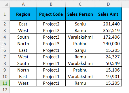

And now, after applying the pivot table, our table will look like this in the figure below.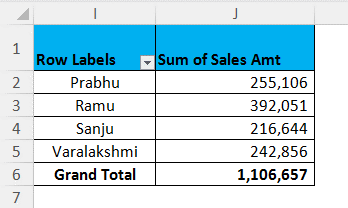

Pro Tips for an individual:We can apply the Getpivotdata function in Microsoft Excel in two ways.

One is primarily done by just clicking out the equal sign (=) in any particular cell (apart from the pivot table cell). Then after that we will select the desired cell in the pivot table field.

Secondly, we will manually enter the Formula just like the other formulas used in Microsoft Excel.

Type 1:Firstly we will be clicking on any particular cell, and then after that, we will select the desired outcome cell in the pivot table. And this will eventually give out the value of 2, 16,444 as seen in the below-attached figure.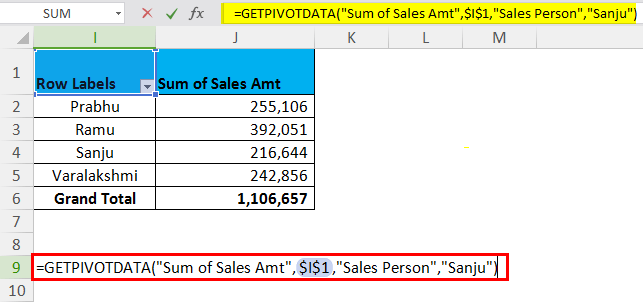

Type 2: Now, in type 2, we will be entering an equal sign on any particular cell in Excel, and then we will enter out the Getpivotdata function effectively, as seen in the below-attached figure.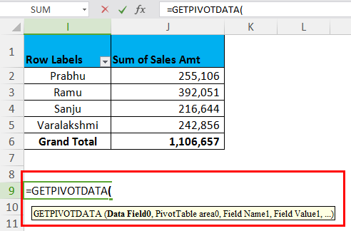

After that, in the respective Data_Field section, we will type"Sales Amt". And in the Pivot Table section, we will type "I1" (the reference cell where our Sales Amt resides, and here, in this case, it is I1).

Furthermore, in the [Field 1] section, we will now type "Sales Person", and in the [Item1] section, we will be organizing "Sanju>". And this will give us a value of 2, 16,444 respectively, as depicted in the screenshot below.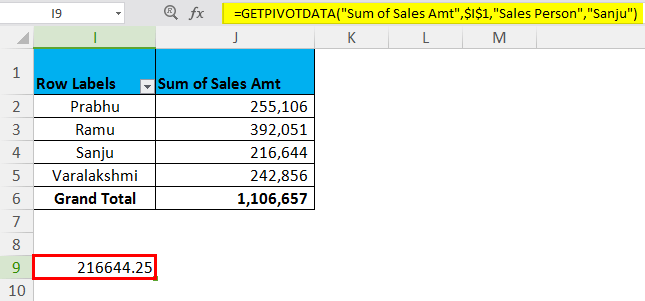

# Example 2: Getting out the Pivot Table Sub Totals in Excel

And for this example we are making use of the same data table which we have used earlier. Still, in these data, we will also insert the pivot table below to use the multi-criterion Getpivotdata function in Microsoft Excel. After all, our pivot should look like this, as seen in the below figure.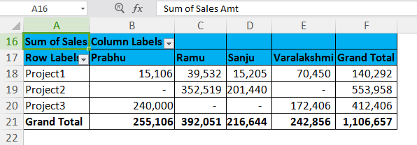

After that, the requirement is to get Mr Ramu's value for Project 2.

=GETPIVOTDATA ("Sales Amt",$A$20, "Project Code", "Project2", "Sales Person", "Ramu"), as depicted in the below-attached figure as well.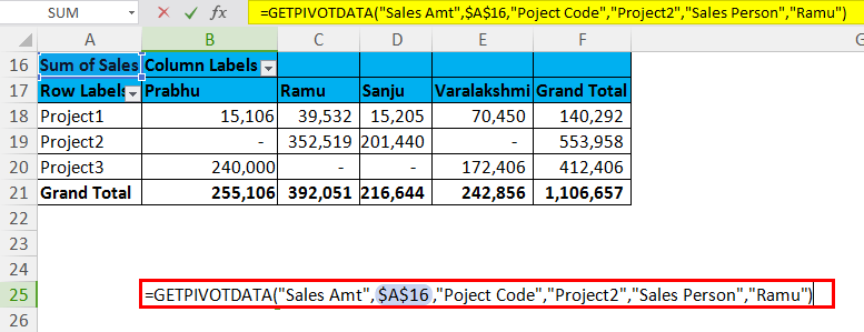

1. Data_Field: Data_Field in Microsoft Excel is used to efficiently enter the Sales Amt data.
2. Pivot_Table: The Pivot_Table in Microsoft Excel is the Cell reference of Sales Amt.
3. [Filed1] & [Item1]: In these, the Project Code is filed out, which we are looking for, and under the project code, which we are looking for, Project 2, respectively.
4. [Filed2] & [Item2]: And in these, the Sales Person is filed; and under this, we are looking for Ramu (Item) effectively.

This means that we are effectively looking for the total sales amount of Mr Ramu for Project 2, respectively, as was seen in the below-attached figure.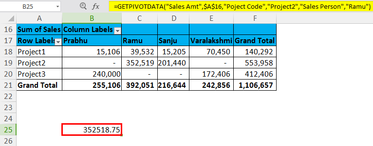

After that, it was requested to note down the overall sales for Mr Ramu, which is none other than the value of 3, 92,051, but for Project 2, the value is 3, 52,519, as seen in the below-attached screenshot.

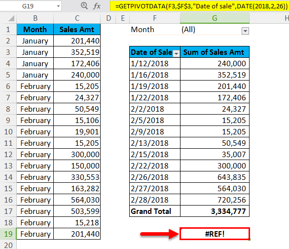
Example #3

In this example, below is the monthly sales data for the Company XYZ, and with the use of the pivot table, we can easily find out the Total Sales Amount for the Date that is 26-02-2018, as can be seen in the below-attached screenshot respectively.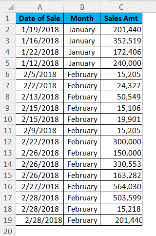

Pivot Table Fields & Values

1. First, we will map out the pivot table for the data as mentioned above.
2. And then assign Date to the Row Data respectively.
3. And eventually, the Value Field should be present in the Sales Amt.

And now, after that, the Pivot Table will look like this, as seen in the below-attached figure.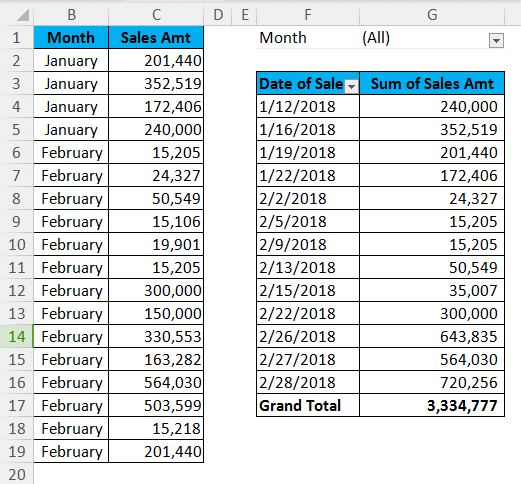

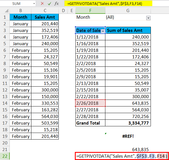
And now, after that, with the help of this table, we can easily find out the sale of 26^thFeb 2018.

And in order to get a correct outcome or the result while typing a date then we should follow the below mentioned formula that is the Getpivotdata Formula.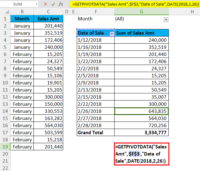

And now the sale of 26^thFeb 2018 is 643835.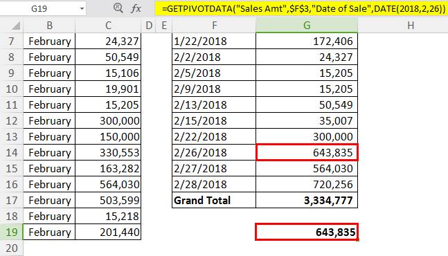

Important Things to Remember

The various vital things or the points which are supposed to be remembered by any particular individual who all are working with the GETPIVOTDATA Function in Microsoft Excel are as follows:

1. The important things to be remembered is that it is not possible to change the first argument of the function in any manner, that is, the Data_Field, to a cell reference; and if we were doing it forcefully, then, in that case, the result or the outcome will throw an error as#REF, so this should be avoided by every respective individual, as depicted in the below-attached figure.
   
2. And the other point is that, by default, Microsoft Excel will take the date format as DATE (2018, 2, 26). But if an individual wants different date format then it is possible by just entering the Date in "dd-mm-yyyy" format, i.e. "26-02-2018", respectively.
3. And it was well known that the function will eventually return #REFerror if an individual supplies the incorrect Data_Field.
4. And all the respective characters of the syntax should begin with double quotes (") and must be ending with the same with no minor difference.
5. Moreover, apart from the Data_Field for all the remaining out fields, we can give or provide a cell reference, so it will give the same result, as was clearly depicted in the figure below.
   
6. And the respective calculated fields (items), and also the the custom calculations, are part of this particular function.
7. All the fields must need to be visible to get the desired result or the outcomes. And if in case the data is not visible, then in that particular scenario, the function will efficiently be returning out the #REF error type.
8. And this particular function will work across the Grand Total and all the Sub Total of the Pivot Table, respectively.