How one can compare two columns for matches and differences in Microsoft Excel?

Introduction to compare two columns in Microsoft Excel

It was well known that the comparison of the respective two columns in Microsoft Excel reached the values in those columns. We have encountered different methods to achieve this.

In the very first way, we can easily select out the parallel cells of the columns which we want to compare it by just separating them by making use of the equal sign ("="), as this will give us the outcome as TRUE or FALSE. And if a cell of the columns is matched, then in that particular case, we will get a TRUE as an output, else FALSE.

Besides all this, in the other way, we can also make use of the IF function for the purpose of matching out the column cells the way we do by just putting out an equal sign in order to get the message which we want when columns are compared.

Now in this tutorial, we will be then exploring out the several techniques for the purpose of compare two columns in Microsoft Excel and then finding matches and differences between them as well.

How one can compare two columns in Microsoft Excel row-by-row?
How one can compare multiple columns for row matches?
How can one compare two columns for matches and differences in an Excel sheet?
How can one compare two lists and pull matching data in Microsoft Excel?
How do highlight matches as well as differences between the two columns?
How can one highlight row matches and differences in an Excel sheet?
How one can compare two cells in Microsoft Excel?
The formula-free way to compare two columns or the list in Microsoft Excel

How we can compare two columns in Microsoft Excel row by row?

If in case we are performing the analysis of data in Microsoft Excel, then one of the most frequent tasks which can be used for the purpose of comparing out the data in each row. And this task can be effectively done by making use of the IF -FUNCTION, as it was demonstrated in the following examples:

#Example 1: Comparing of two columns for the matches or differences in the same row

For the purpose of comparing out the two columns in Microsoft Excel row-by-row, we will be writing usual IF formula in order to reach the first two cells. We will be then entering the formula in another column in the same row and then copy it to other cells by just dragging the fill handle. As we do this, the cursor changes to the plus sign effectively:

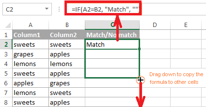
How one can compare two columns for matches and differences in Microsoft Excel?

Formula that can be used for matches in Microsoft Excel

The formulas which can be used for the purpose of matching in the Excel sheet are as follows:

And in order to find out the cells within the same row having the same content, A2 as well as the B2 in this example,

=IF (A2=B2,"Match","")

Formula that can be used for the differences in Microsoft Excel

The formulas which can be used for the purpose of finding out the differences in the Excel sheet are as follows:

And for the purpose of finding out the cells in the same row with the various values, replace the equals sign with the non-equality sign (<>),

=IF (A2<>B2,"No match","")

Matches and differences

Moreover, nothing prevents us from finding both matches as well as the differences with a single formula as well:

=IF (A2=B2, "Match," "No match")

=IF (A2<>B2, "No match," "Match")

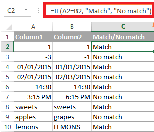
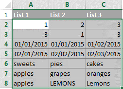
As we can see that, the formula handles out the numbers, dates, times, as well as the text strings.

Important note: We can also compare the row-by-row columns using the Excel Advanced Filter.
Let us now we will be seeing an example of how to filter matches as well as the differences between the two columns.

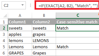
#Example 2: How to comparing the two lists for case-sensitive matches in the same row in the Excel sheet

As we have noticed that, the formulas from the previous example will be ignoring the case when we compare out the text values, as in row 10 in the screenshot above. If in case we want to find out the case-sensitive matches between the 2 columns in each row, then we will be making use of the EXACT function effectively:

=IF (EXACT (A2, B2), "Match", "")

And for the purpose of finding out the case-sensitive differences in the same row, we will be then entering the corresponding text ("Unique" in this example) in the 3^rd argument of the IF function, e.g.:

=IF (EXACT (A2, B2), "Match," "Unique")

How to compare the multiple columns for matches in the same row in the Excel sheet?

In our Microsoft Excel worksheets, the multiple columns can be compared which are based on the following criteria:

How one can find out the rows with the same values in all columns given in Microsoft Excel? (Example 1)
How one can find rows with the same values in any 2 columns in Microsoft Excel? (Example 2)

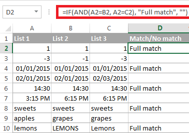
# Example 1: Finding out the matches in all cells within the same row in the Microsoft Excel

If in case our table has 3 or more columns and we want to find out the rows that have the same values in all cells, an IF formula with an AND statement will work as a treat:

=IF (AND (A2=B2, A2=C2), "Full match", "")

If in case our table has a lot of columns, then a more elegant solution would be to make use of the COUNTIF Function:

=IF (COUNTIF ($A2:$E2, $A2) =5, "Full match", "")

In which 5 is the number of the columns which we are comparing?

# Example 2: Finding out the matches in any two cells in the same row in an Excel sheet

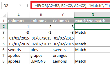
If we are looking for a way that can be used to for the purpose of comparing out the columns for any two or more cells with the same values within the same row by just making use of an IF formula with an OR statement:

=IF (OR (A2=B2, B2=C2, A2=C2), "Match", "")

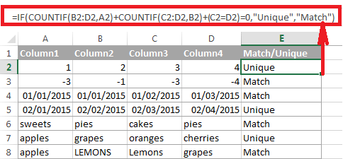
And if many different columns can be used for the purpose of comparing then our OR statement may grow too big. So in this case, a better solution would be just adding up the several COUNTIF functions. And the first COUNTIF counts how many columns have the same value as in the 1^st column respectively, whereas the second COUNTIF counts how many of the remaining columns are equal to the 2^nd column. If the count is 0, the formula will return a "Unique" or "Match" respectively.

For example:

=IF (COUNTIF (B2:D2, A2) +COUNTIF (C2:D2, B2) + (C2=D2) =0,"Unique","Match")

How to compare the two Microsoft Excel columns for matches and differences?

We are generally having a 2 lists of data in Microsoft Excel, and with which we want to find all the values which are present in column A but not in column B as well.

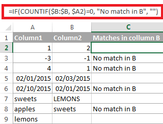
And for this, we can embed out the COUNTIF function in IF's logical test and will then check if it returns zero or any other number.

For instance, the following IF or the COUNTIF formula searches across the entire column B for the value in cell A2. If in the case when no match is found, then the formula will return "No match in B."

=IF (COUNTIF ($B: $B, $A2) =0, "No match in B", "")

And the same result can also be achieved by making use of an IF formula with the embedded ISERROR and MATCH functions effectively:

=IF (ISERROR (MATCH ($A2, $B$2:$B$10, 0)), "No match in B," ")

Or, by just making use of the following array,

=IF (SUM (--($B$2:$B$10=$A2)) =0, "No match in B", "")

If in case we want a single formula for the purpose of identifying both matches (duplicates) as well as the differences (unique values), put some of the text for matches in the empty double quotes ("") in any of the above formulas respectively.

For example:

=IF (COUNTIF ($B: $B, $A2) =0, "No match in B," "Match in B")

How to compare two lists in Microsoft Excel and pull matches in an Excel sheet?

Sometimes we just need to match two columns in two different tables and pulling out the matching entries from the lookup table. Microsoft Excel will also provide a unique function for this - the VLOOKUP function. And as an alternative, we can use a more robust and versatile INDEX MATCH formula, and the users of Excel 2021 and Excel 365 can also accomplish the task with the XLOOKUP Function.

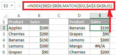
For example, The following formulas will then compare the product names in column D that are against the names in column A and pull out a corresponding sales figure from column B if a match is found; otherwise, the #N/A error is returned respectively:

=VLOOKUP (D2, $A$2:$B$6, 2, FALSE)

=INDEX ($B$2:$B$6, MATCH ($D2, $A$2:$A$6, 0))

=XLOOKUP (D2, $A$2:$A$6, $B$2:$B$6)

How can one compare the two lists and highlight matches and differences in the Excel sheet?

When we are comparing the columns in Microsoft Excel, if in case we may want to "visualize" the items which are efficiently present in one column but missing in the other one as well, we can shade such cells in any color of our own choice by making use of the Microsoft Excel Conditional Formatting feature. The below-mentioned examples will demonstrate the detailed steps as well:

# Example 1: Highlighting matches and differences in each row

Now in this, to compare the two columns and the Microsoft Excel and highlight the cells in column A that will have identical entries in column B in the same row, do the following as well:

Step 1: First, we will select the cells we may want to highlight (we can determine the cells within one column or in several columns if we're going to color entire rows) respectively.

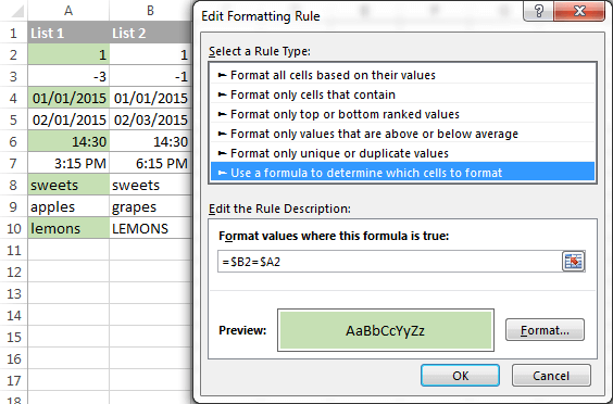
Step 2: After that, we will click on the Conditional formatting > New Rule? > Use a formula to determine which cells to format as well.

Step 3: After that, we will create a rule with a simple formula like =$B2=$A2 (assuming that row 2 is the first row with data, not including the column header). And then, we will double-check that we have made use of a relative row reference (without the $ sign) like in the formula above respectively.

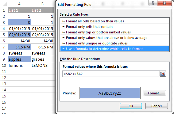
Now to highlight the differences between columns A and B, as it will be creating a rule with this formula as well:

=$B2<>$A2

# Example 2: Highlight unique entries in each list in the Excel sheet

Whenever we are comparing the two lists in Microsoft Excel, there are 3 item types that we can highlight respectively:

Items that are only in the 1^st list (unique)
Things that are only on the 2^nd list (special)
Items that are in both lists (duplicates).

This example will demonstrate how to color the items only in one list.

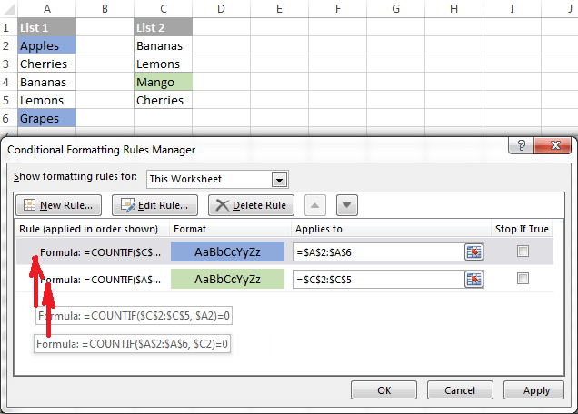
Our List 1 is in column A (A2: A6) as well as the List 2 is present in column C (C2: C5). We can also create conditional formatting rules with the following formulas:

Highlighting out the unique values in List 1 (column A):

=COUNTIF ($C$2:$C$5, $A2) =0

Highlighting unique values in List 2 (column C):

=COUNTIF ($A$2:$A$6, $C2) =0

And get the following result as well:

# Example 3: Highlight out the matches (duplicates) between 2 columns in the Excel sheet

If we closely followed the previous example, we could adjust the COUNTIF formulas so that they find the matches rather than the differences. All of us have to do is just to set the count greater than zero respectively:

Highlight out the matches in List 1 (column A):

=COUNTIF ($C$2:$C$5, $A2)>0

Highlight out the matches in List 2 (column C):

=COUNTIF ($A$2:$A$6, $C2)>0

How can one highlight row differences and matches in multiple columns in Microsoft Excel?

When we are comparing values in several columns row-by-row, then the quickest method that can be used to highlight the matches is just by creating a conditional formatting rule, and the fastest way to shade differences is embracing the Go To Special feature, which is efficiently demonstrated in the following examples as well:

# Example 1: Comparing out the multiple columns and highlight row matches

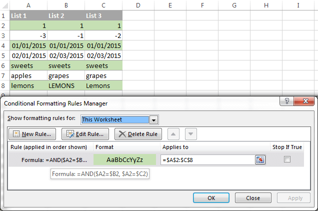
To highlight the rows that have identical values in all columns, we need to create a conditional formatting rule which is based on one of the following formulas as well:

=AND ($A2=$B2, $A2=$C2)

=COUNTIF ($A2:$C2, $A2) =3

A2, B2, and C2 are the top-most cells, and 3 is the number of columns used for the comparison.

Of course, neither AND nor the COUNTIF formula is limited to comparing only 3 columns. We can use other similar formulas to highlight rows with the same values in 4, 5, 6, or more columns.

# Example 2: Comparison of the multiple columns as well as highlighting the row differences in Excel

If we want to quickly highlight the selected cells with different values in each row, we can use Excel's Go to Special feature, respectively.

Step 1: First of all, we will be selecting out the range of the cells which we want to compare, and in this example, we have selected the cells that is from A2 to C8, respectively:

By default, the top-most cell of the selected range is the active cell, and the cells from the other selected columns in the same row will be compared to that particular cell. As we can see in the above screenshot, the active cell is white, while all other cells of the selected range are highlighted as well. As in this example, the active cell is A2, so the comparison column is column A only.

And if we want to change the comparison column, we can use either the Tab key to navigate through selected cells from left to right or the Enter key to move from top to bottom.

Important tip: For the purpose of selecting out the non-adjacent columns, we will select the first column, pressing as well as holding the Ctrl, and then selecting the other columns. The active cell will be in the last column (or the last block of adjacent columns). And to change the comparison column, we use the Tab or Enter key as described above.

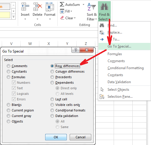
Step 2: Now, on the Home tab, we will go to the Editing group, and then click on Find & Select > Go to Special, then select out the Row differences and click the OK cbutton as well.

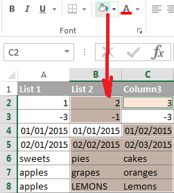
Step 3: The cells whose values differ from the comparison cell in each row are colored. If we want to shade out the highlighted cells in some color, we can click the Fill Color icon on the ribbon and select the color of our choice.

How can one compare two cells in Microsoft Excel?

Comparing 2 cells is a case of comparing two columns in Microsoft Excel row by row, except that we do not have to copy the formulas to other cells in the column.

For example: For comparing the cells A1 and C1, we can use the following formulas.

For matches:

=IF (A1=C1, "Match", "")

For differences:

=IF (A1<>C1, "Difference", "")

Formula-free way to compare two columns/lists in Microsoft Excel

Let me show our solution now that we know that Microsoft Excel's offerings are for comparing and matching columns. And this tool is named that is Compare Two Tables, and it is included in our Ultimate Suite.

The add-in can compare two tables or lists by any number of columns. Both identify matches or differences (as we did with formulas) and highlight them (as we did with conditional formatting, respectively.

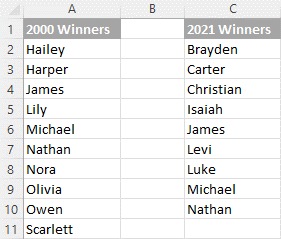
For this purpose of this, we will be comparing the following 2 lists in order to find common values that are present in both.

And to compare the two lists, here are the steps which we need to follow as well:

Step 1: First, we will click the Compare Tables button on the Data tab.

Step 2: Then we will be selected the first column/list and click Next. In terms of the add-in, this is your Table 1 respectively:

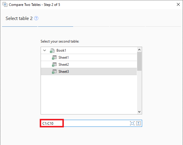
Step 3: Now we will be selected the second column/list and click Next. In terms of the add-in, it is our Table 2, and it can reside in the same or different worksheet or even in another workbook as well:

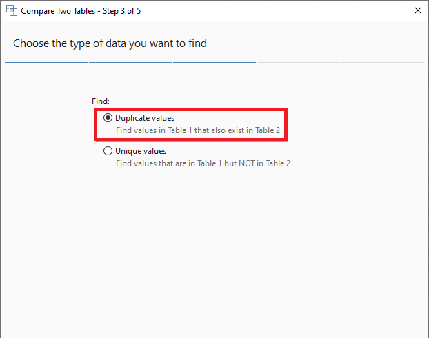
Step 4: Choosing what kind of data to look for:

Duplicate values (matches) - the items that exist in both lists.
Unique values (differences) - the items in list 1 but not list 2.

As our main aim is to find the matches, we will select the first option and click on Next.

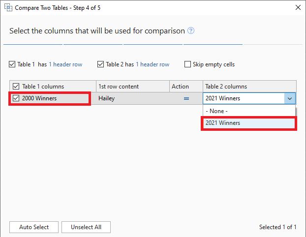
Step 5: This is crucial to select the columns for comparison. In our case, the choice is evident as we are only comparing 2 columns: 2000 Winners against 2021 Winners. In bigger tables, we can select several column pairs to compare by as well:

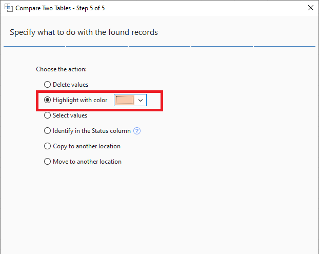
Step 6: In the final step, we must choose how to deal with the found items and click the Finish button.

A few different options are available here. For our purposes, these two are most helpful:

Highlight with color - shades match or differences in the selected color (like Excel conditional formatting does).
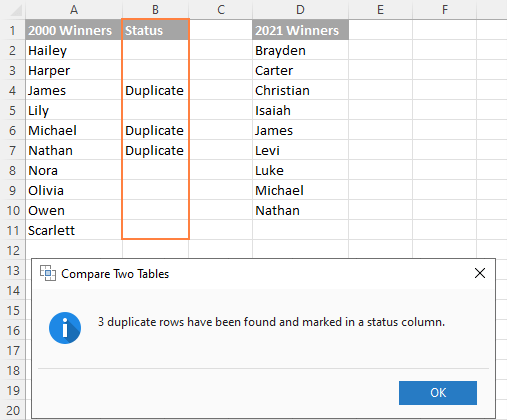
Identify in the Status column - inserts the Status column with the "Duplicate" or "Unique" labels (like IF formulas do).
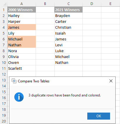
For this example, I've decided to highlight duplicates in the following color: