How one can sum only filter cells in Microsoft Excel

Introduction to Filter in Microsoft Excel

In Microsoft Excel, the term "Filter" is primarily used for the purpose of displaying the relevant data by just eliminating the irrelevant entries on a temporary basis from the respective view. And the particular data is being filtered in accordance with the given criteria by an individual as well.

Moreover, the main purpose of filtering data or the cells is mainly used to focus on the various crucial areas of a dataset.

• For example, the sector-wise sales data for a particular given organization can be easily filtered by the given location. Hence, the user can efficiently view the sales of a selected sector at a given interval of time.

Besides, a filter is required while working with a huge set of databases. And being one of the widely used tools, the particular filter converts a comprehensive view into an easy-to-understand one. And if we need to apply filters, the dataset must contain a header row specifying the name of every column respectively.

In this tutorial, we will be discussing the three important methods which can be used to calculate the sum of the filtered cell in Microsoft Excel, which are as follows:

1. Use of SUBTOTAL Function to sum only filtered cells in Excel?
2. Use of Aggregate Function in Microsoft Excel.
3. Use of the User-Defined Function in Microsoft Excel.

How to make use of the SUBTOTAL FUNCTION in Microsoft Excel?

It was well known that the respective "SUBTOTAL function" is primarily used for the purpose of calculating a subtotal in a given dataset. And some of the importance of this Function is that, it will present out various options which can be basically used to perform calculation of totals such as:

• Sum.
• Average.
• Maximum value as well as the minimum value.

And the SUBTOTAL Function gives 2 options that can be used to calculate a sum;

1. The very first of them will be working just like the "SUM function".
2. And the other one is totaling of the visible cells, which is our target.

Syntax: The syntax which can be used for the SUBTOTAL Function in Microsoft Excel is as follows:

In which:

1. Function_num: The Function_num is primarily a number that is ranging from 1 to 11 or 101 to 111, specifying which functions need to be just used for the subtotal.
2. Ref1, Ref2, The cells or ranges which we want to subtotal effectively. And the first Ref is an essential one and it can't be ignored.

The below mentioned formula which is purposely used for the purpose of summing the visible cells by just making use of the SUBTOTAL Function effectively:

Formula:

In this, the very first argument is none other than the function number. Moreover the number as well as its relevant functions is given while entering the SUBTOTAL Function. Then we will be finding out the two options for sums; 9 and 109.

And the Function number 9 is the option for the SUM function, whereas the number 109 will also be working for the manually hidden cells respectively.

After then we will be selecting 109 from the given options, so the SUBTOTAL function basically totals out the values of the selected filtered cells: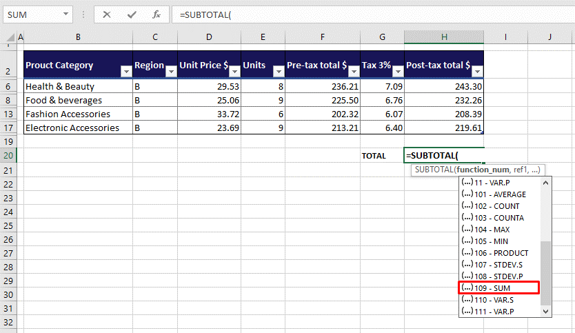

Nextly for the second argument, we can just start referring to the individual cells for the summation purpose. And we have selected our visible cells that will automatically become H6:H17.

Now we will have our result: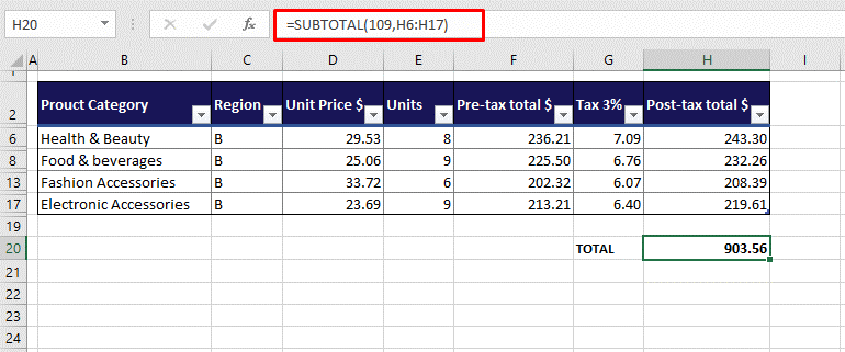

So now this Function will be effectively working well for the hidden rows, and it does not work for the hidden columns. And if in case there is a presence of any hidden row along with the Range that are referred in the formula, then in that case their respective values will not be included in the given result of the "SUBTOTAL function". But if there is a presence of any hidden column, so unfortunately those particular values can easily make their way to the SUBTOTAL's result.

How to make use of the Aggregate Function in Microsoft Excel?

The AGGREGATE function returns an aggregate in a particular database in Microsoft Excel. So the question is: How is it different from the SUBTOTAL Function?

So some of the basic differences between the two for the purpose of returning a summation are that they both work in a similar fashion but only in case of the AGGREGATE function, we can handpick those things which we want to be get included or excluded from the total.

Now we will be seeing the working of the AGGREGATE function that it will be returning the sum of the visible cells. First of all, we will be using the below-mentioned formula:

Formula:

As with the SUBTOTAL Function, we will first enter the function number. Here in this scenario, we will be assuming number 9 for summation.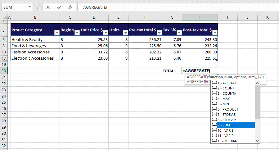

Next, we will get the options for the values ignored by the Aggregate. In this example, we need to have the values in the filtered rows, by just making option 5 as: ignore hidden rows a good fit.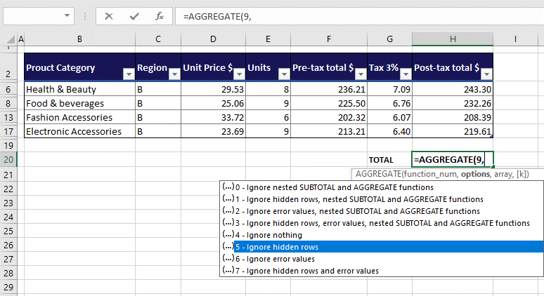

Now, for the particular array. We have entered out H6:H17.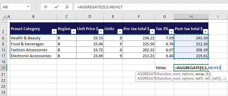

And the AGGREGATE function has ignored all the hidden rows in order to sum the values that are visible in the Range that is H6:H17.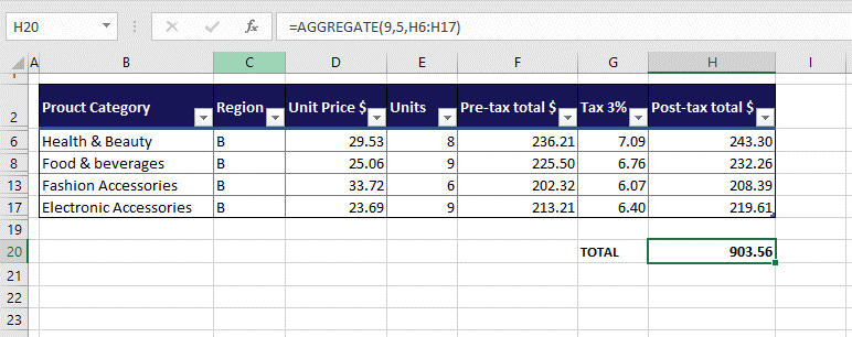

In this it should be noticed that how the options in the formula only mention the hidden rows and not the columns. Why? The reason is that the AGGREGATE function primarily does not work for hidden columns as well.

Making use of the User-Defined VBA Function in Microsoft Excel

In this method, we will be working with a user-defined function in order to get the sum of the visible cells. No, we cannot just go by creating functions in Microsoft Excel at our whim; it is because of the reason that we will need to have VBA as well as a VBA code.

The code can be used through the VBA so to create the Function, and then the Function could be used on the particular worksheet as like all other functions effectively.

Why do we go through the bother of creating a function? We will need help leaving out the hidden columns in the SUBTOTAL as well as in the AGGREGATE functions. But in this VBA function, we can have the Function to leave out the hidden rows as well as the columns.

Here is how we are going to make use of the user-defined Function in VBA (Virtual Basic for Application) for the summation of a visible cell as well:

Step 1: First, we will be pressing out the Alt + F11 keys in order to launch the VB, or if we have the Developer Tab added, we can go to the tab Code group and click on the Visual Basic button.

Step 2: Once the VB editor is open, we will then click on the Insert tab and select Modulefrom the given list.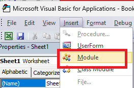

Step 3: In the given Modulewindow, we will be copying and also pasting the code to add the Function as well:

And then, a function will get created with the name "SumVisible" that can be used to calculate the total of the selected cells visible in the given data set while ignoring the values in the hidden rows and the columns.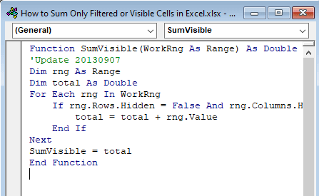

Step 4: After that, we will be closing the VB.

Step 5: Now, in the cell where we want the total, we will be entering the following formula as mentioned below:

And we only need to enter the created function name and the Range. Then the Function will sum out all the values given in the Range and will return the total: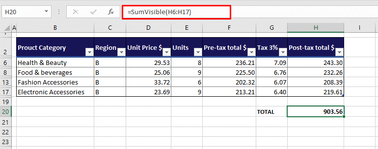

Note: It should be noted that the given values in hidden rows as well as in the columns shall be left out from the calculation. Do note, however once the particular formula has been entered, and if we are needed to hide a row, then the result will adjust to exclude the value hidden effectively. But if in case we hide a column, we are needed to recalculate the formula.

We can recalculate by just selecting the cell with the given formula, and going into cell edit mode, pressing the Enter key.