How to add a hyperlink to another worksheet

Hyperlinks have immense value in the Internet world. It holds the capability to instantly redirect to other information in just a single click. The same concept is used in Microsoft Excel to hyperlink your spreadsheets. Spreadsheet Hyperlinks is a great tool that has plenty of advantages.

In this tutorial, we will unveil the real-time use of spreadsheet hyperlinks and the step-by-step tutorial on inserting them into your Excel worksheets. We will also cover the steps to change a link destination and modify its format. If you don't require the hyperlink any more in your worksheet, you'll see how to remove it.

We will be covering the following topics:

1. What is a Spreadsheet hyperlink?
2. Insert a hyperlink in Ms Excel
   • Method 1: To insert the hyperlink from the context menu
   • Method 2: Using Excel HYPERLINK function
   • Method 3: Insert a link by cell drag-and-drop
3. Edit a hyperlink
   • Change the Hyperlink destination
   • Modify hyperlink format
4. Remove a hyperlink

What is a Spreadsheet Hyperlink?

"Spreadsheet Hyperlink allows the user to access an external worksheet in your system. If you create internal hyperlinks in your spreadsheet, they can help you to quickly link only the necessary part of the workbook without scrolling multiple worksheets."

In Microsoft Excel there are three types of hyperlinks that are as follows:

1. Link your worksheet to an existing or to a new file
2. Link your worksheet to a web page
3. Link the data to an e-mail address

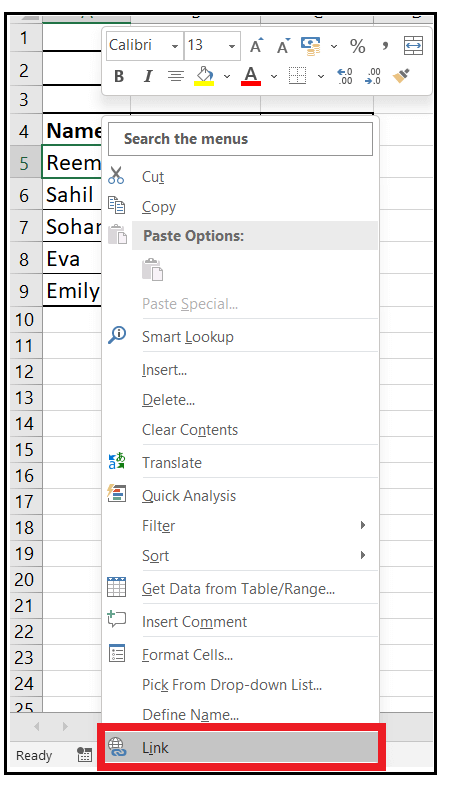
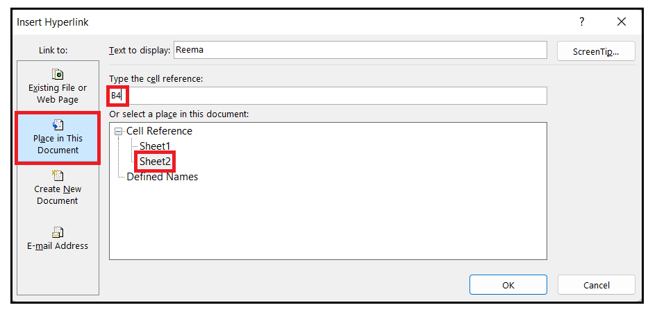
You can choose any one of the above depending upon your requirement.

Insert a hyperlink in Ms Excel

Microsoft Excel provides different ways to insert a hyperlink in your workbook. In this section, we will cover three methods to add a hyperlink to your Excel worksheet to easily navigate between different workbooks.

Method 1: To insert the hyperlink from the context menu

You can use this method if you want to add a hyperlink within one workbook. It uses the Hyperlink command to insert the hyperlink.

Following are the steps:

1. Point your mouse cursor to select a cell where you want to add your hyperlink.
2. The next step is to right-click on the cell and from the appeared context menu choose the Hyperlink or Link option.
   
3. The Insert Hyperlink window will be displayed on the screen.
4. If you want to link the cell to a particular location within the same workbook, choose the Place in This Document in the Link to section.
5. Select the worksheet that you want to link to in the Or select a place in this document field.
6. End the cell address in the given cell reference box. Doing so will link to the selected cell to the specified cell address of another worksheet.
7. Type the value or the content in the Text to display field box. This data will represent the hyperlink in the cell.
   
8. To complete the process, click on OK button. You will get the following output.
   

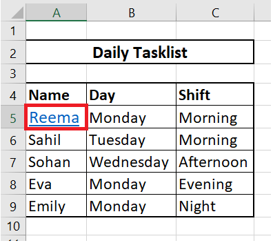
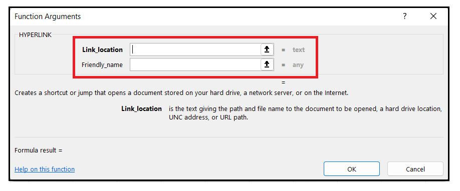
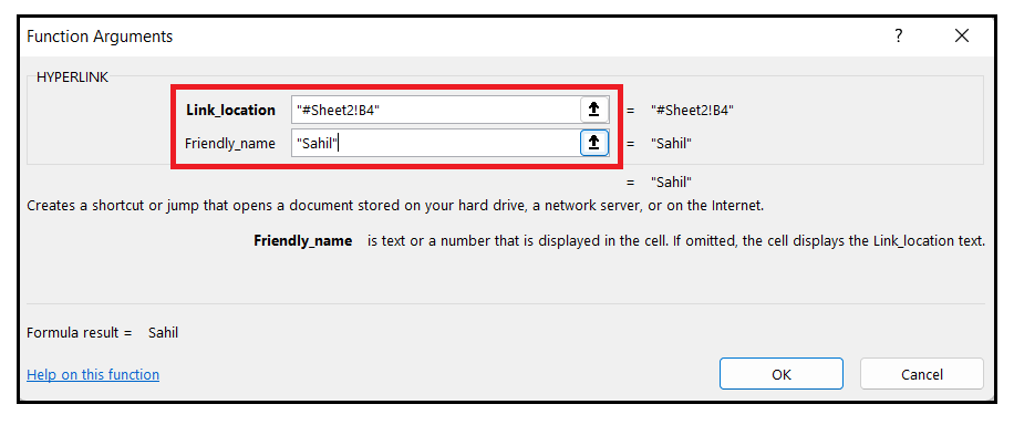
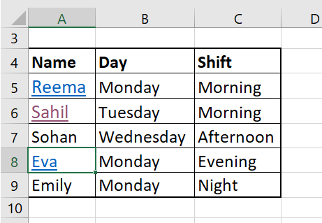
As soon as the hyperlink process is completed, the selected cell's data gets underlined and highlighted in blue. Such an impression indicated that the cell contains the hyperlink. To quickly crosscheck whether the hyperlink works, just hover the pointer over the underlined text and click on it. As a result, it will jump and redirect you to the specified location.

Method 2: Using Excel HYPERLINK function

Microsoft provides different functions to help us in our day-to-day Excel works. One such function is the HYPERLINK function. As the name suggests, it helps the users to quickly create links between spreadsheets in the workbook. If are someone who loved exploring different function, do the following:

1. Point your mouse cursor to select a cell where you want to add your hyperlink.
   
2. From the formulas tab, go to the function library option and select the Lookup & Reference option.
   
3. The following drop-down list will appear. From the Lookup & Reference drop-down select the HYPERLINK option.
   
4. As soon as you do that, the Function Arguments window will appear. All you need to do is to type two HYPERLINK function arguments in the given window: link_location and friendly_name.
   Refer to the below screenshot:
   
5. The link_location window refers to a specific cell from which you want to link your data. Here we will specify the hyperlink destination. In our case, we have selected the cell B6 in sheet2.

Note: If you have no idea what destination cell address to put in, you can use the Select range icon to manually select the linking cell.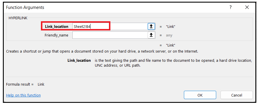

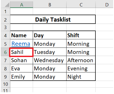
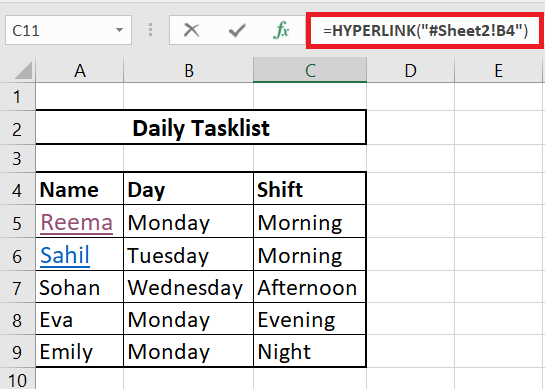
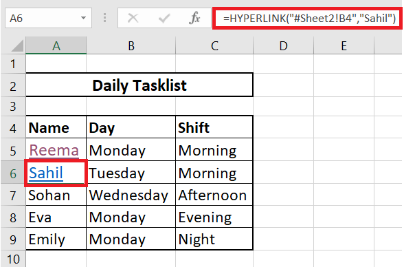
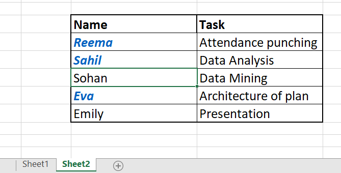
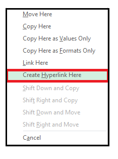
1. Make sure to add the # sign (number symbol) before the given location.
   
2. The second field, i.e., friendly_name, represents the jump text clicking on, which will take you to the liked cell. Enter the Friendly_name you want to display in the cell, and put it in double quotes.
   
3. Once done click on the OK button.
   

You are all done! To your surprise, the text is hyperlinked, and if you click on the cell, you can see the formula in the formula bar. Click on the linked cell to take you to the destination cell.

Method 3: Insert a link by cell drag-and-drop

As the name suggests, drag-and-drop method is one of the easy and quickest method to add a hyperlink in your workbook. In this section let's cover how it is done!

In this example, we are given two sheets, therefore we will create a hyperlink in Sheet 1 to a cell in Sheet 2.

Note. This method doesn't work in new workbooks, so ensure your workbook is saved before starting the steps.

1. Put your cursor and select the hyperlink destination. In our case, we have selected B4 cell in Sheet 2.
2. Move your cursor to the borders of the selected cell and right-click.
   
3. Hold the cursor and move down to the sheets tab.
4. Press the Alt key to move over the to the Sheet 1 tab.

NOTE: Pressing the Alt key helps you to move your data to the next sheet. You can release the button once Sheet 1 is activated.

1. Drag the cursor to the cell where to want to add the hyperlink.
2. Click the right mouse button and the following menu will be displayed. From the menu, choose the Create Hyperlink Here option.
   
3. The hyperlink is created to the cell when you select the above option. To cross-check, click on the cell, which will directly take you to the destination cell in Sheet 2.

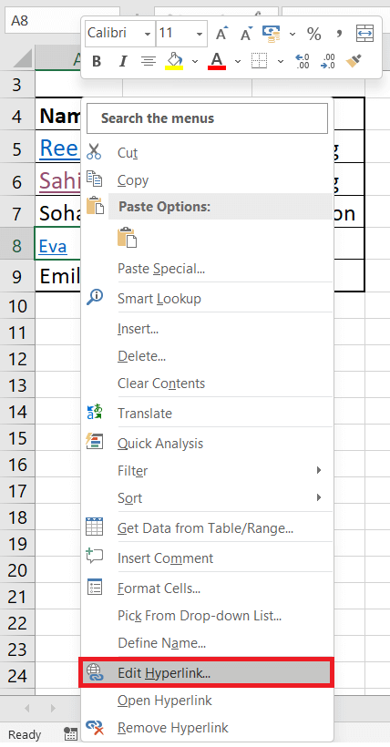
The results are evident. Dragging is the fastest option among the suggested methods. It saves time by joining multiple operations into a single task. It might take less time but needs more attention when compared with the other two methods. One single mistake and you might end up getting the wrong results.

Choose any option that suits you well, and keep creating your hyperlink!

Edit a hyperlink

Editing a hyperlink is an interesting option that enables the user to change the link destination or the appearance of the text used to represent it. Let's capture both methods in this section:

Change the Hyperlink link destination

So far, we have covered different methods to add hyperlinks to various spreadsheets within the same workbook. But what if you release that you have inserted the wrong hyperlink, or you, due to any reason, want to change the hyperlink destination? You can modify the cell reference or choose another sheet following some easy steps given below:

1. The first step is to right-click on the existing link you want to edit.
2. The pop-up menu will appear. Choose the Edit Hyperlink from the menu.
   
3. The Edit Hyperlink will be displayed. However, you will notice that this window looks identical to the Insert Hyperlink window and contains the same fields and layouts.

Note. You can also open the Edit Hyperlink panel by pressing the shortcut key Ctrl + K or from the Insert Group, choose the Hyperlink option. Make sure to select the linked cell before opting any method.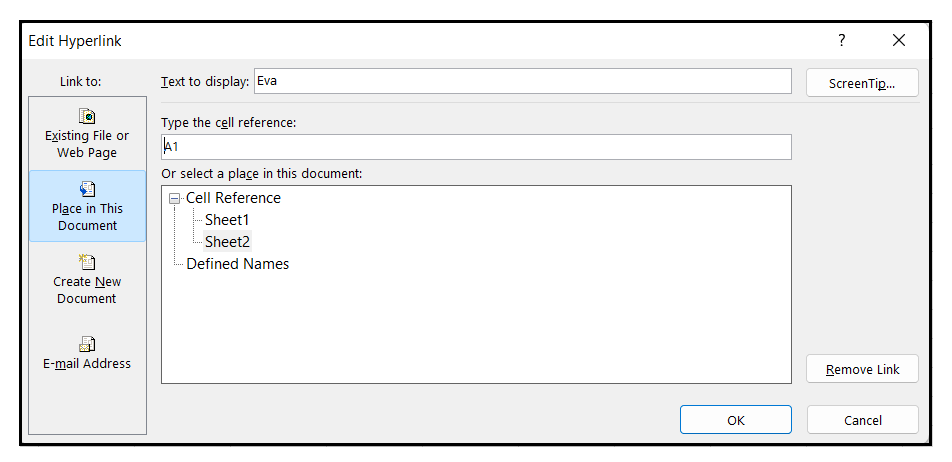

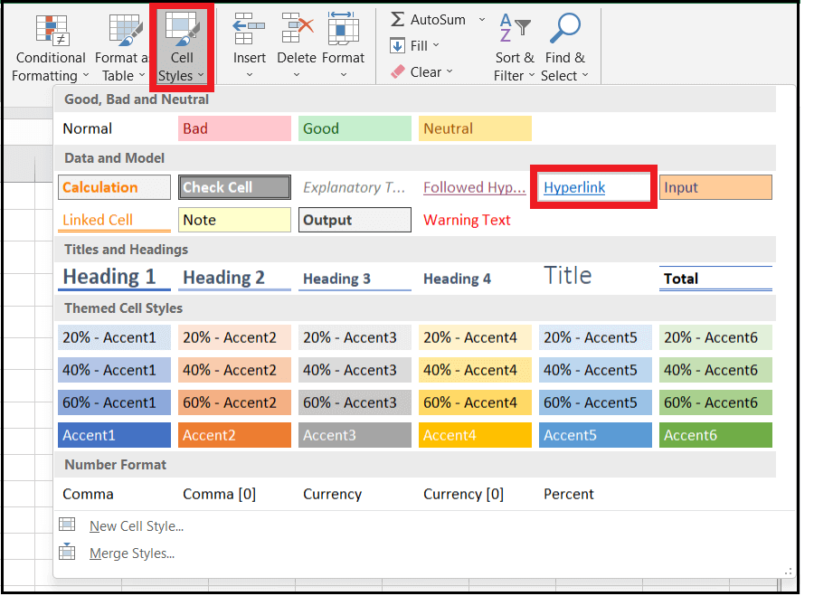
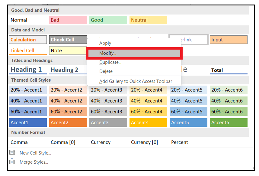
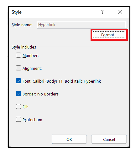
1. From the Cell Reference you can select and change the sheet name. In the Type the cell reference field, enter the cell address.
2. Click on the OK button to lock the changes.
   

It will edit the cell reference, and now if you click on Eva instead of jumping to cell B4 of Sheet2, it will move to cell A4 of Sheet2.

Modify hyperlink format

The default text appearance of a hyperlink is underlined, and it is present in shades of blue. But if you want to be creative and persistent in changing the typical appearance of a hyperlink, you can easily modify it to stand out from the crowd. Follow the below steps to adjust the hyperlink format quickly:

1. Click on the HOME tab and select cell styles option from the styles group. It will open the Cell Styles list.
2. Look for the hyperlink option and right-click on it. If your hyperlink is already active you can also right-click on the Followed Hyperlink option.
   
3. From the appeared menu select the Modify option.
   
4. The styles dialog window will pop up. Click on the Formation option.
   
5. In the format cells window, do the required changes. Fill color, change font or you can add an alignment to the hyperlink text.
6. Once you are done, click on OK button.
7. Press the OK button once again and you will notice the hyperlinks appearance has changed to the latest ones.
   

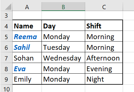
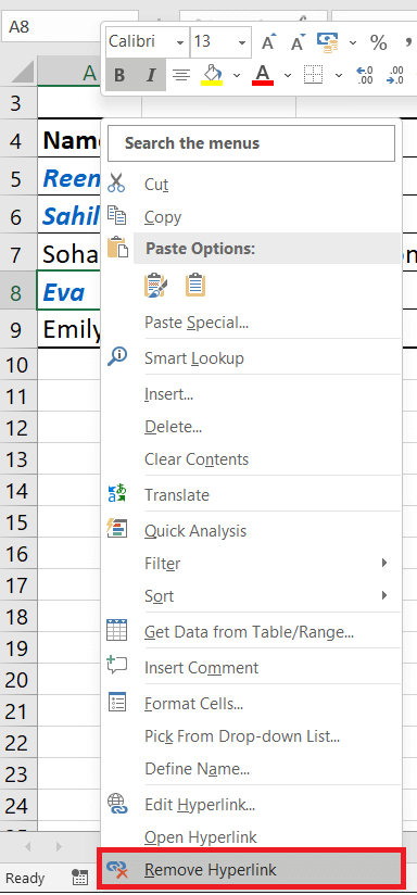
Enjoy unique and new styles of hyperlinks in your Excel workbook. Kindly note that the changes you made are in effect for all the hyperlinks in the workbook; you can't simply change the style of a single hyperlink.

Wasn't that simple? Following some simple steps, you can easily customise the appearance of a hyperlink in Microsoft Excel.

Remove a hyperlink

So far we covered the methods and steps to add, edit and modify hyperlink. But what about if we want to remove it? Deleting a hyperlink is super easy as it only takes couple of seconds and zero to remove the hyperlink from the worksheet.

All you need to do is to follow the below steps:

1. Select the hyperlink that you want to delete and right-click on it.
2. The window will appear. From the listed options click on the Remove Hyperlink option.
   
3. You will notice that the underline and blue text mark has been disappeared from the text. It means the text remains in the cell, but the hyperlink has been removed.

Note. If you want to delete a hyperlink as well as the text that represents it, select the cell that contains the link and right-click on it. From the appeared menu, choose the Clear Contents. It will do the needful.