How to extract text from Excel cells?

Excel is widely used for office and personal use. It consists of enormous functions and formulas for the given data, which helps retrieve it quickly and easily. The data entered by the user is either a numeric value, alphabet or mathematical symbol.

Sometimes the data entered by the user is a combination of numeric values and alphabets. Extracting the respective or required text from the data present in the cell manually is a difficult one. To rectify this problem, Excel provides some powerful text functions that help extract the required text from the given data.

What is called a Substring in Excel?

Before explaining the text functions, the concept of "Substring" is explained here for better understanding. A substring is extracting or parsing the string from the combination or group of strings. It is a subset or part of the given string. In general, the example of a substring is as follows,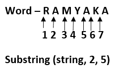

The result will be displayed as AMYAK, the 5 characters from the second position.

Excel Text functions

There is no substring function present in Excel. The various text and default functions are present in Excel to parse the text from the cell. The various text functions are as follows,

Among the various text functions, the main text functions which are used for extracting the text are MID, RIGHT, LEFT, LEN, FIND, REPT, SUBSTITUTE, TRIM and MAX. Some of the text functions are mentioned above in the worksheet. Let's have a look at an example for each Text function.

Example 1: How to extract the middle of the text from the given data?

To extract the middle of the text from the given data, the steps to be followed are,

1. Enter the data in the worksheet, namely A1.
2. Select a new cell and type the formula as =MID (A1, 7, 6). Here A1 indicates the cell name, and 7, 6 indicates that the MID function starts to position the data from the 7^th position and parses the 6 characters.
3. The result will be displayed in the selected cell, which is parsed from the given data.

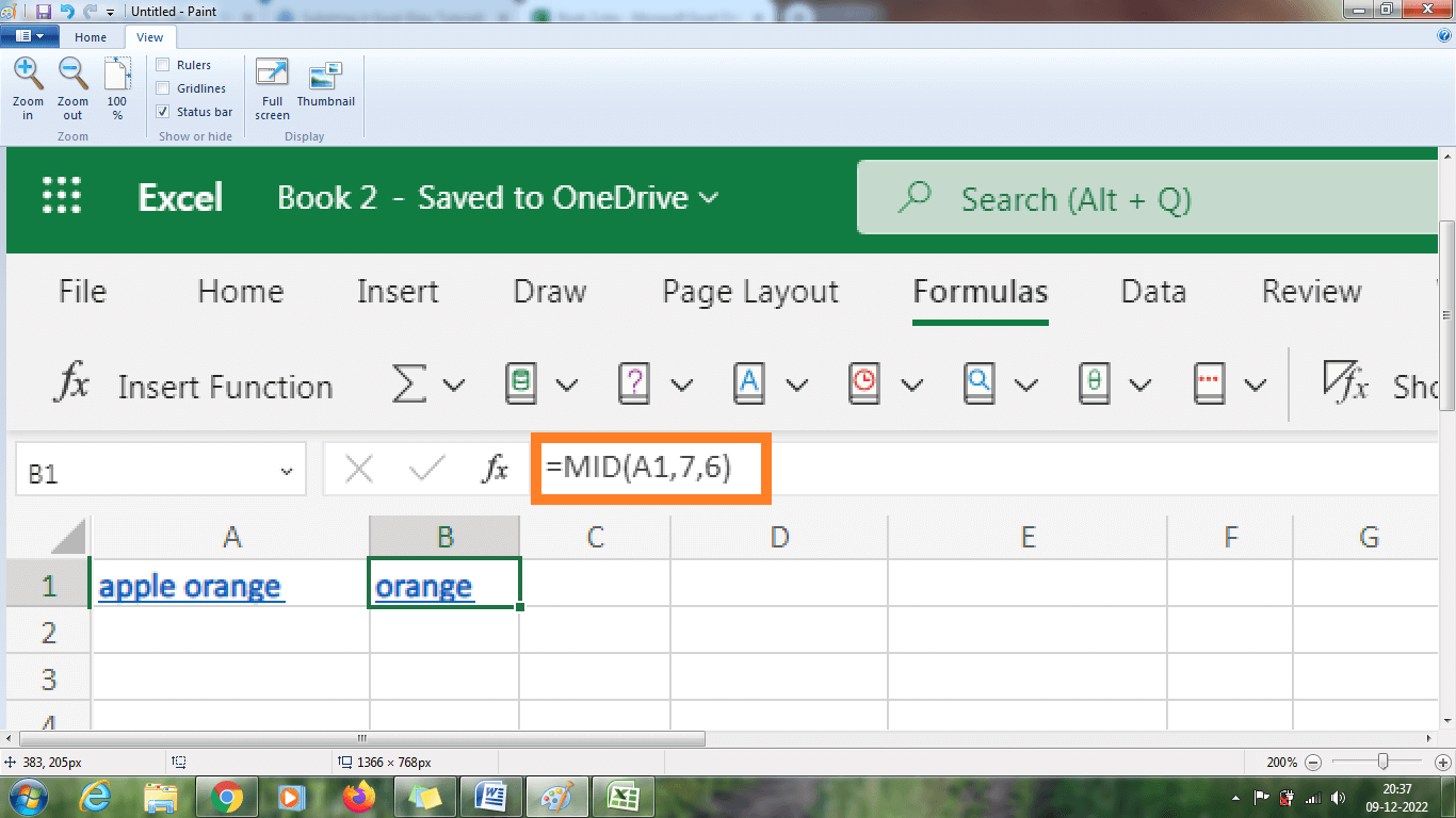
From the above worksheet, the MID function parses the text orange. Here 'o' is mentioned as the 7^th position as the comma is included in the 6^th position.

Example 2: How to extract the left of the text from the given data?

To extract left of the text from the given data, the steps to be followed are,

1. Enter the data in the worksheet, namely A1.
2. Select a new cell and type the formula as =LEFT (A1, 5). Here A1 indicates the cell name, and 5 indicates the count of characters present on the left side.
3. The result will be displayed in the selected cell, which is parsed from the left from the given data.

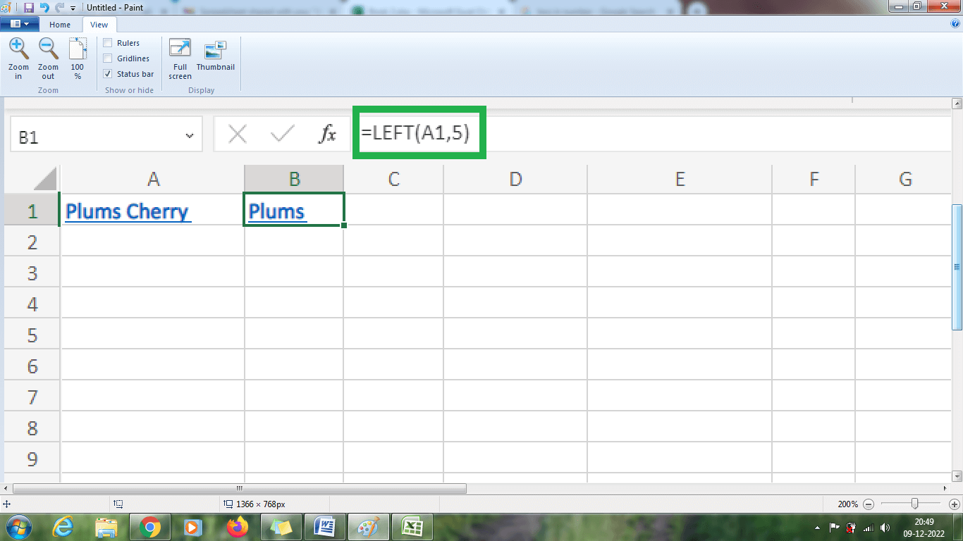
The above worksheet will display the result as plums, five-count characters parsed from the left.

For the same example, the formula can be modified as =LEFT (A1, FIND ("-", A1)-1). The final result will be as same as Plums. Here in this formula, the FIND position finds the position of the "-" and subtracts one from the position of the dash value. The final result will be the position of the leftmost character, which is parsed from the data.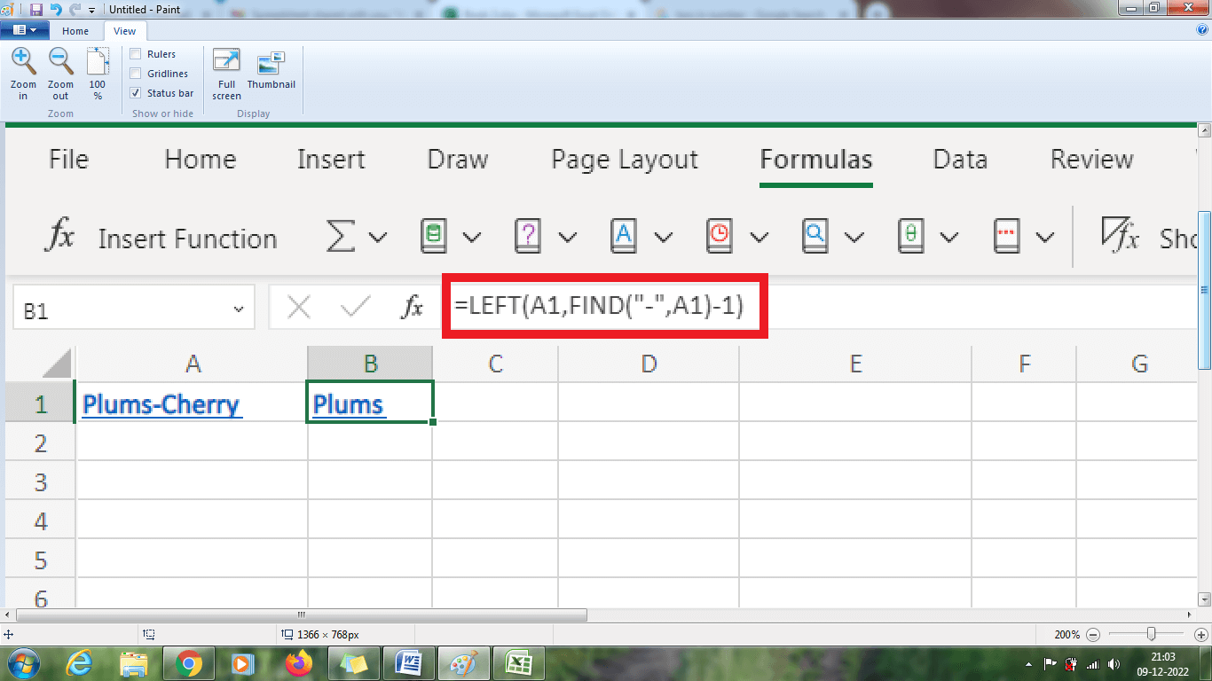

From the above worksheet, the result will be displayed as "Plums" using the FIND function.

Example 3: How to extract the right of the text from the given data?

To extract right of the text from the given data, the steps to be followed are,

Step 1: Enter the data in the worksheet, namely A1.

Step 2: Select a new cell and type the formula as =RIGHT (A1, 6). Here A1 indicates the cell name, and 6 indicates the count of characters present on the right side.

Step 3: The result will be displayed in the selected cell, parsed right from the given data.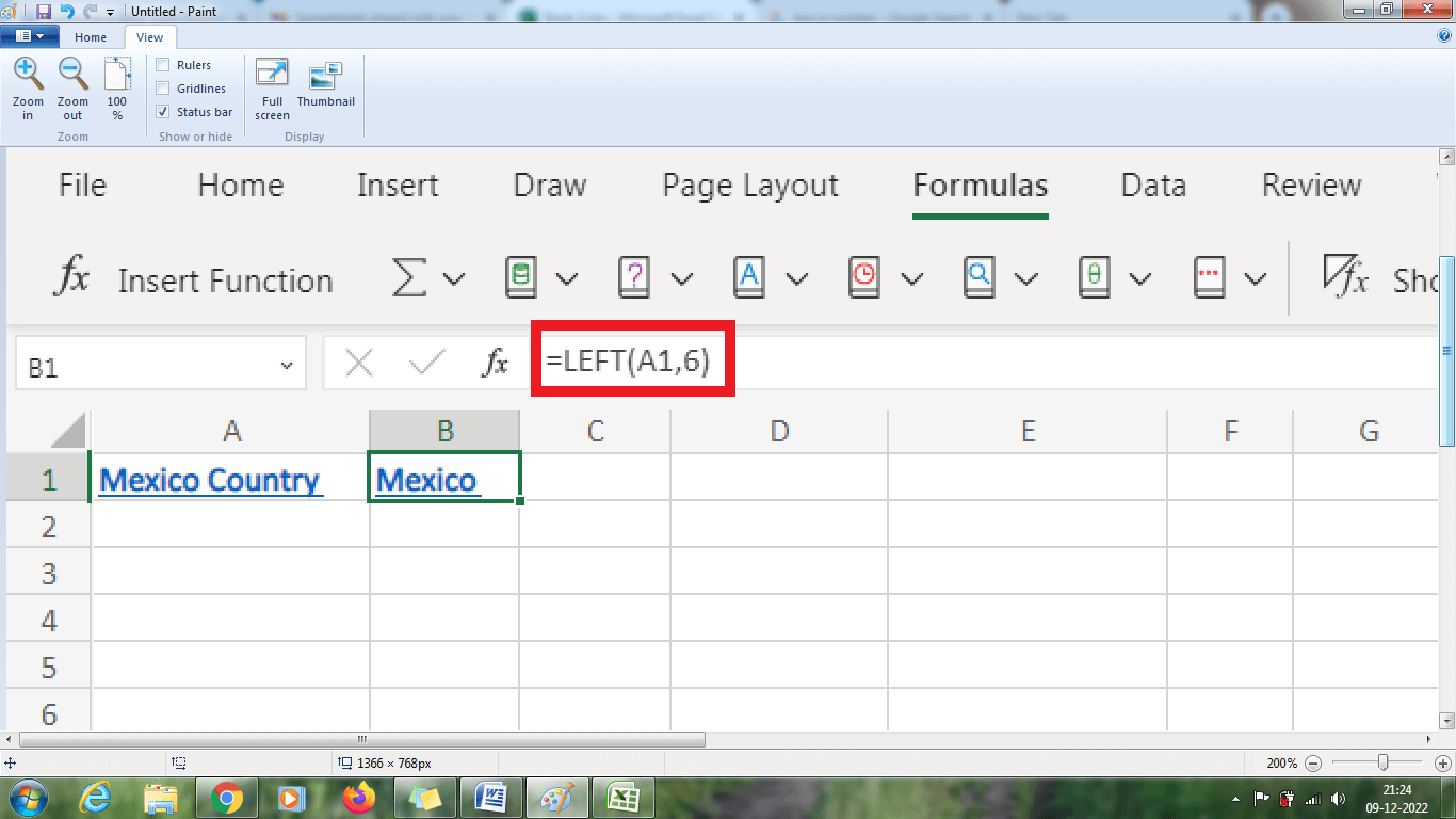

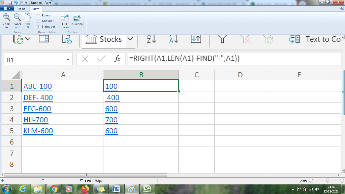
The above worksheet will display the result as Mexico. A six-count character is parsed from the right of the given data.

Example 3.1: How to extract the right of the text present after a dash of any length?

LEN and FIND extract any length of the character present after the dash. The steps to be followed are,

Step 1: Enter the data in the worksheet, namely A1.

Step 2: Select a new cell and type the formula as =RIGHT (A1, LEN (A1)-FIND ("-", A1)). Here LEN function returns the length of the string, and the FIND function finds the position of the dash. Hence from the total length, the position of the dash value is subtracted, and the rightmost character is parsed from the data.

Step 3: The result will be displayed in the selected cell, parsed right from the given data.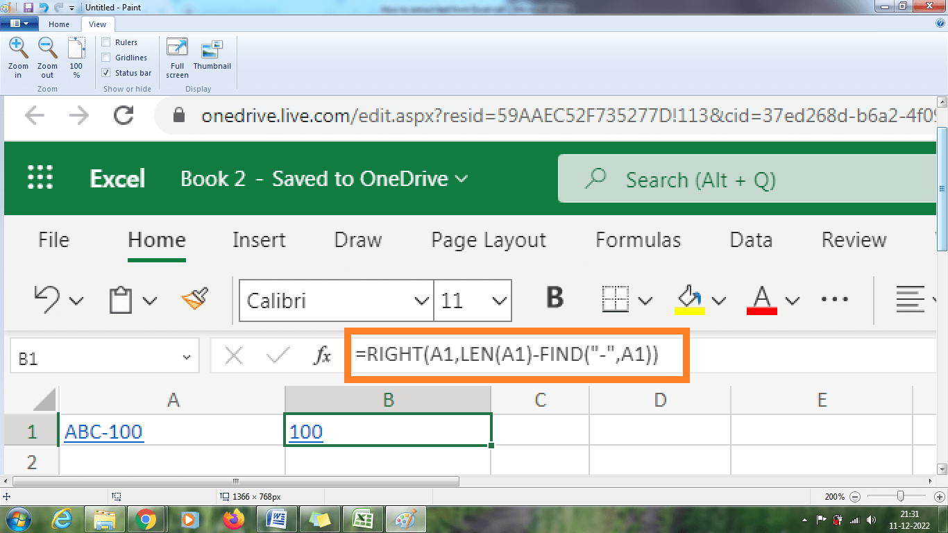

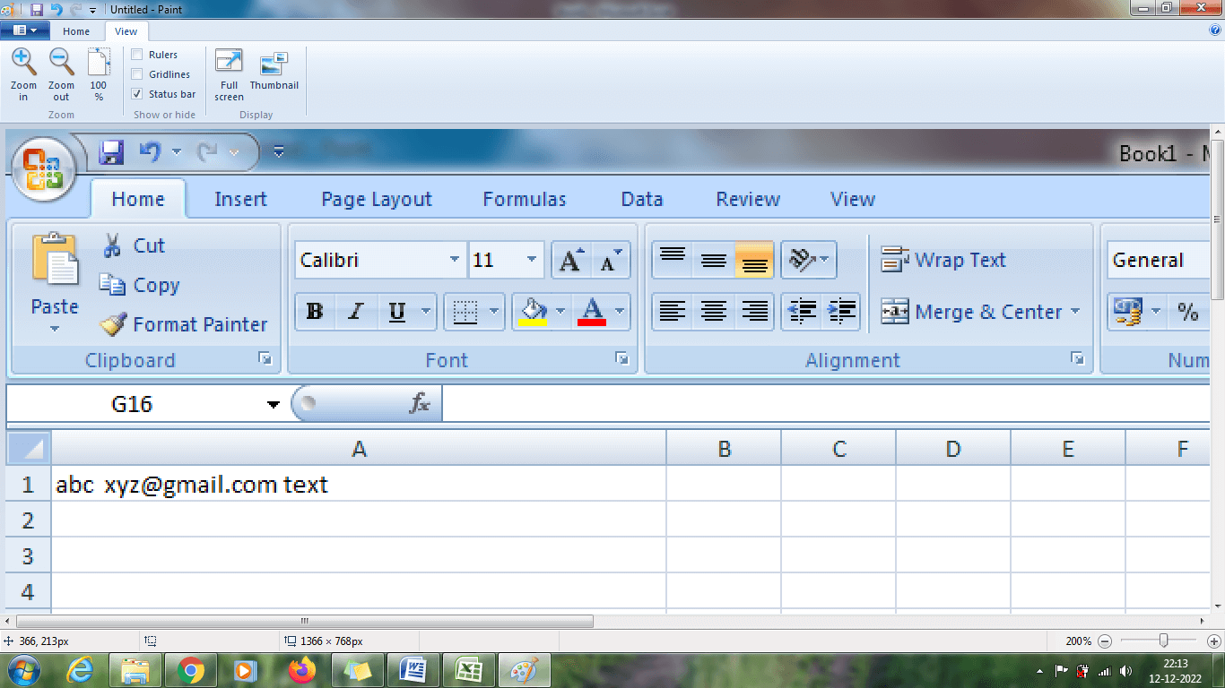
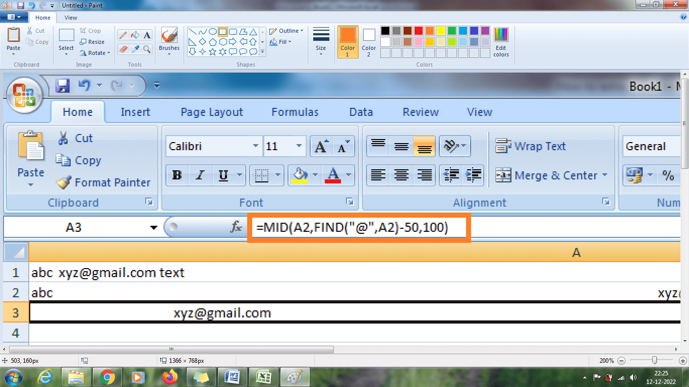
Here the formula returns the total length of the string value as 7 and positions the dash as 4. Hence 7-4= 3. This is parsed from the right of the data.

Example 4: How to extract the username from the mail-id?

Here in this example, the given data set contains various email-ids. The user wants to retrieve the username in a separate cell. The steps to be followed are,

Step 1: Enter the data in the required column A1:A5

Step 2: Identifying the pattern type helps modify the formula more easily and quicker. Here the pattern is '@', which lies between the username and domain name. Select a new cell where the user wants to display the result and type the formula as =LEFT (A1, FIND ("@", A1)-1). The formula uses'@'acts as a reference to get the user name in the separate cell.

Step 3: The result will be displayed in the selected cell, which contains the username of the respective email id.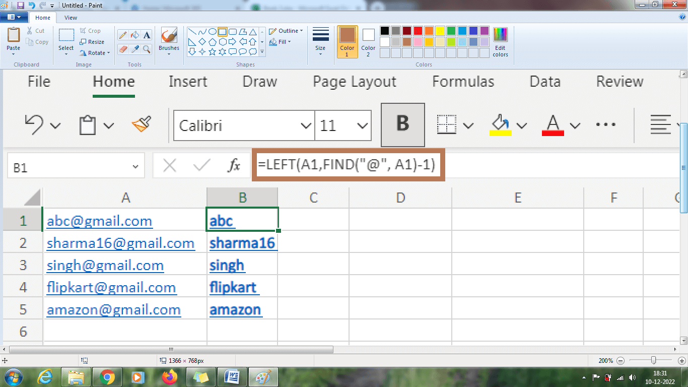

From the above worksheet in cell A1, the FIND function in the formula positions the '@' symbol in the 4^th position and subtracts 1 from it. Hence the result will be 3, which is the count of characters parsed from the left of the given character. Similarly, this method is followed for all the data in the worksheet.

Example 4.1: How to extract the domain name from the mail-id?

In example 3, the username is extracted from the data. The same concept is followed here with a minor difference, and the character is parsed from the data's right side. Here in this example, the given data set contains various email-ids. The user wants to retrieve the domain name in a separate cell. The steps to be followed are,

1. Enter the data in the required column A1:A5
2. Identifying the pattern type helps modify the formula more easily and quicker. Here the pattern is '@', which lies between the username and domain name. Select a new cell where the user wants to display the result and type the formula as =RIGHT (A1, LEN (A1)-FIND ("@", A1)). The formula uses'@'acts as a reference to get the domain name in the separate cell.
3. The result will be displayed in the selected cell containing the respective email ID's domain name.

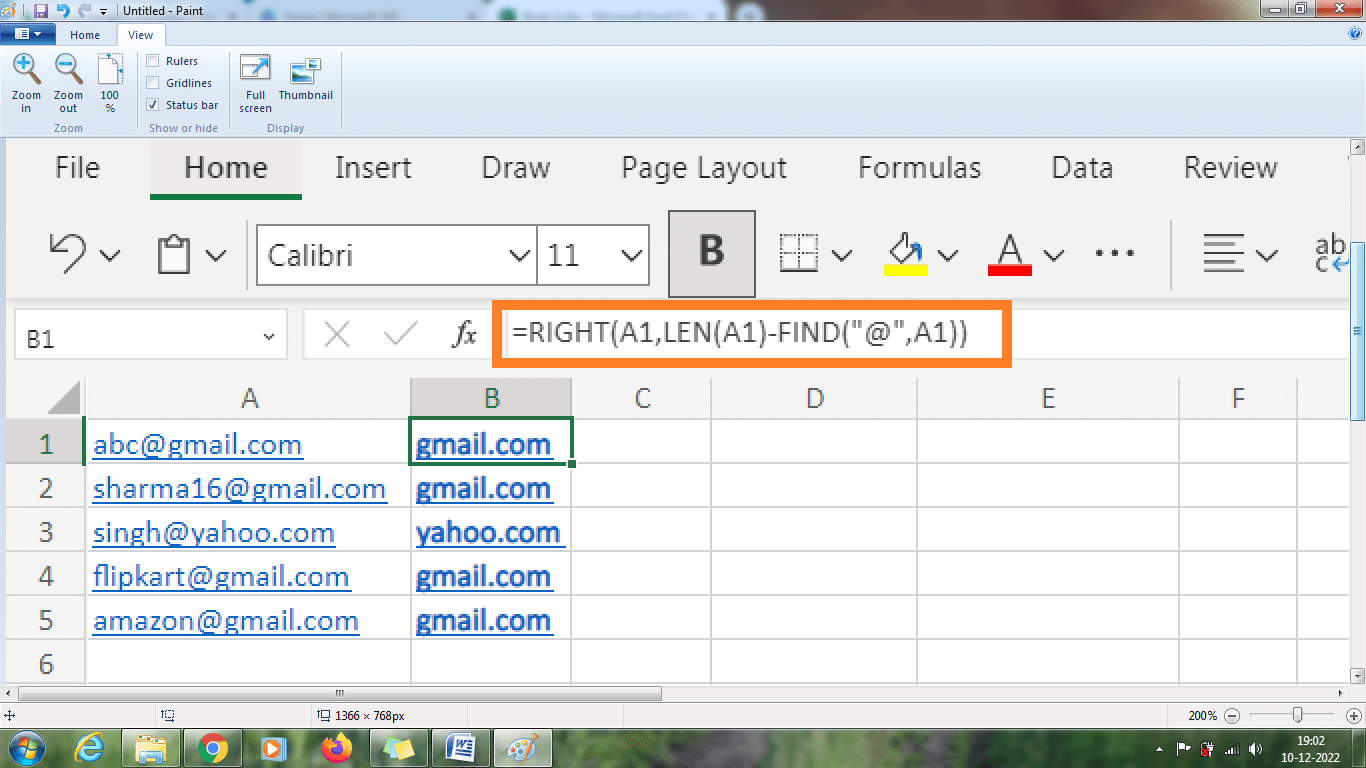
From the above worksheet in cell A1, the FIND function in the formula positions the '@' symbol in the 4^th position. The user wants to extract the character present after the '@' symbol. Hence the total length of the string is founded and subtracted with the character present before the '@' symbol. Finally, the character present towards the right of the '@'symbol is displayed as a result. Similarly, this method is followed for all the data in the worksheet.

Example 5: How to extract the domain name from the mail-id without.com?

To extract the domain name without .com, the formula is modified as follows,

The MID function extracts the specified characters from the starting position from the above formula. FIND ("@", A1) +1 indicates the starting position, right of @. FIND (".", A1)-FIND ("@", A1)-1) counts the character between '@' and '.'

The steps to be followed are,

Step 1: Enter the required data in column A1:A5

Step 2: Select a new cell where the user wants to display the result and enter the formula as =MID(A1, FIND("@", A1)+1, FIND(".", A1)-FIND("@", A1)-1)

Step 3: The result will be displayed in the selected cell, which is the domain name without .com.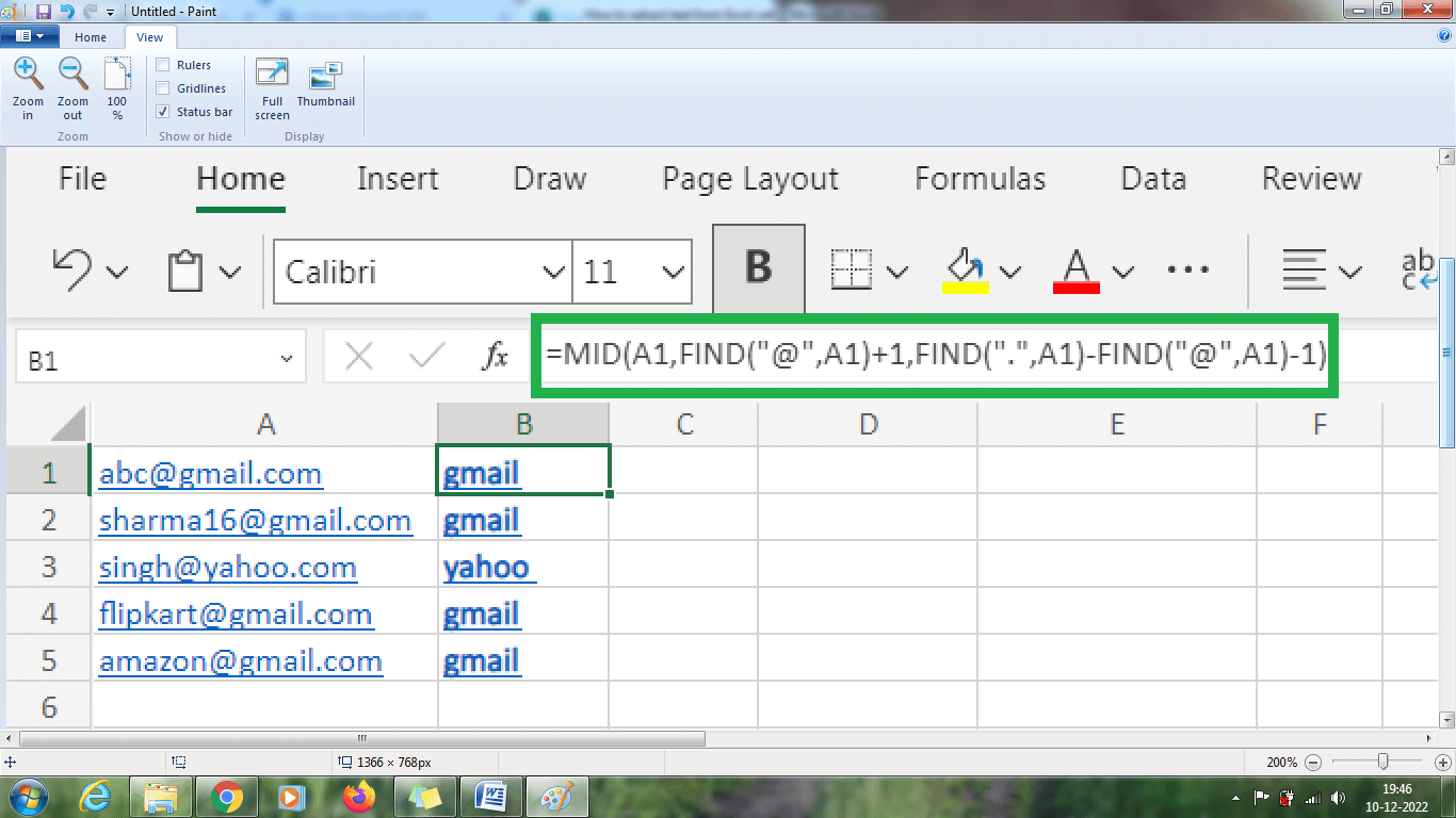

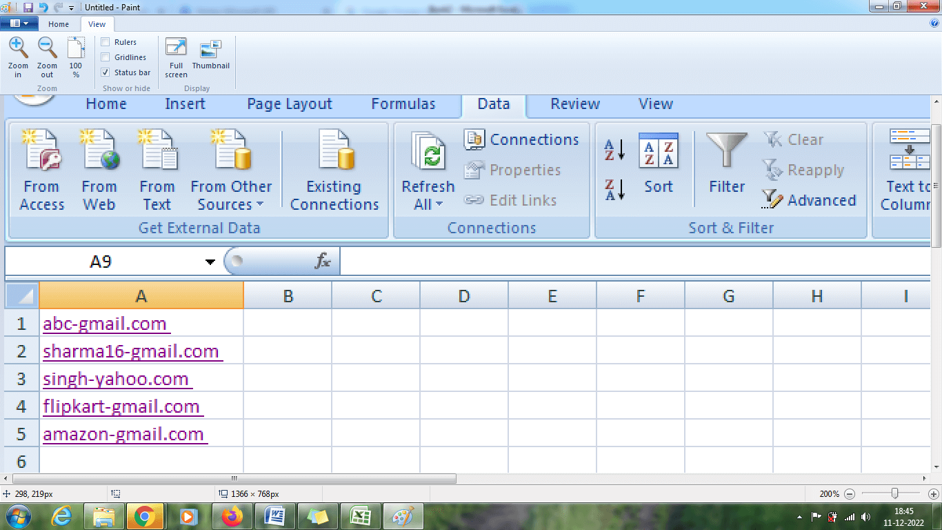
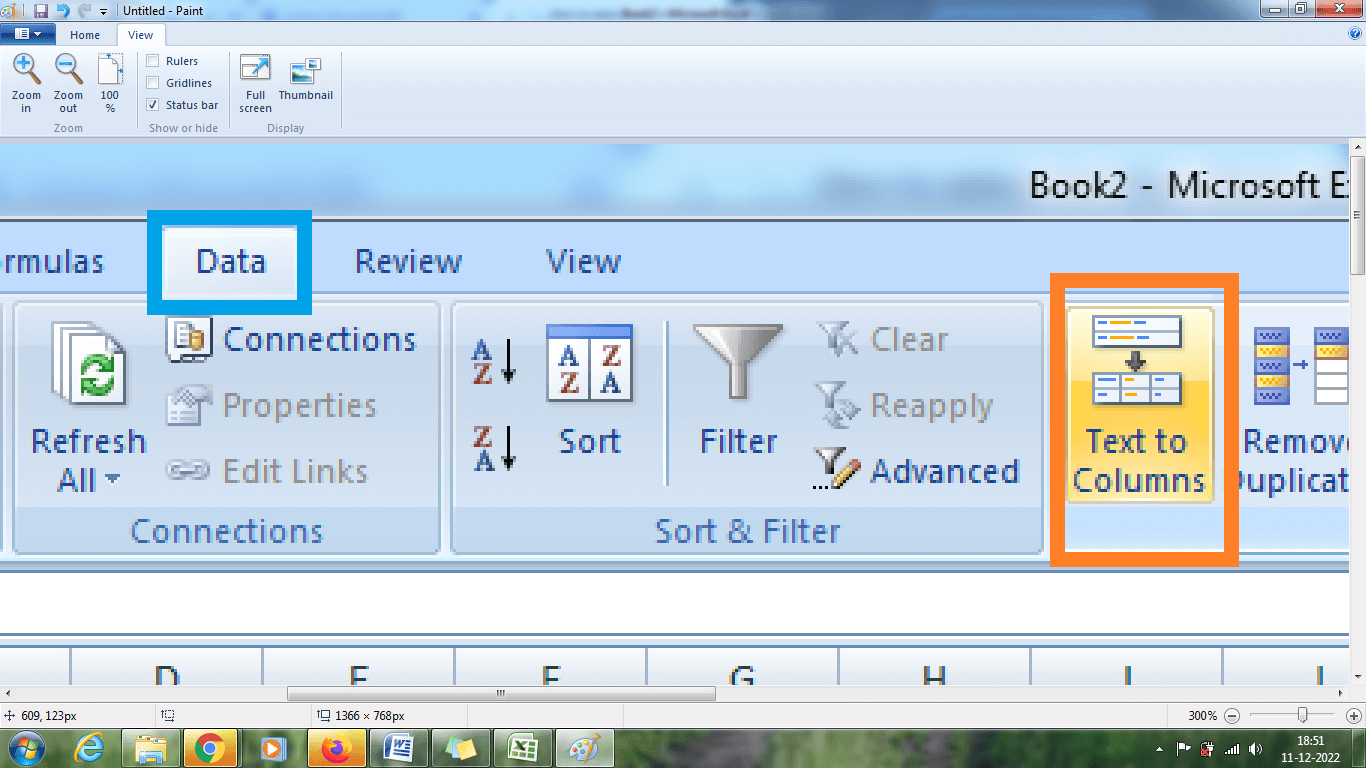
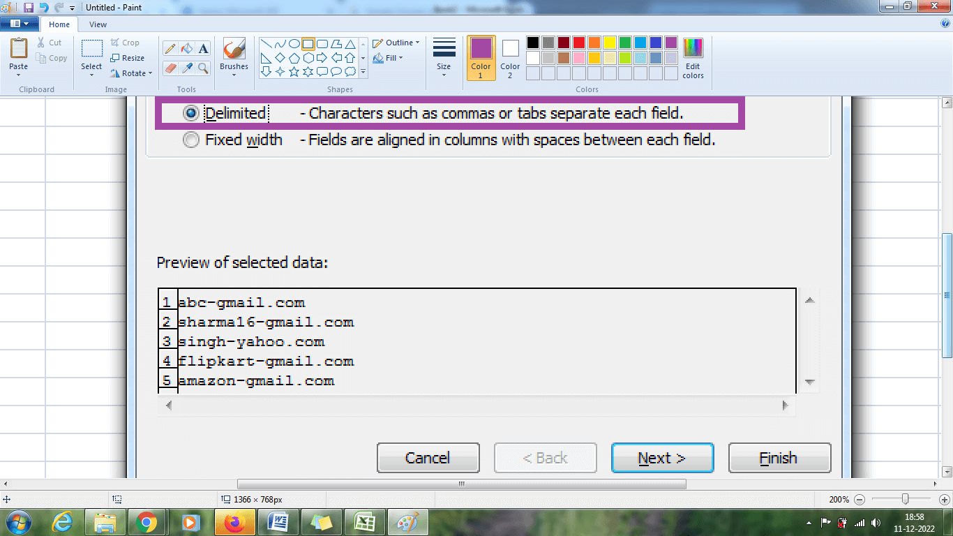
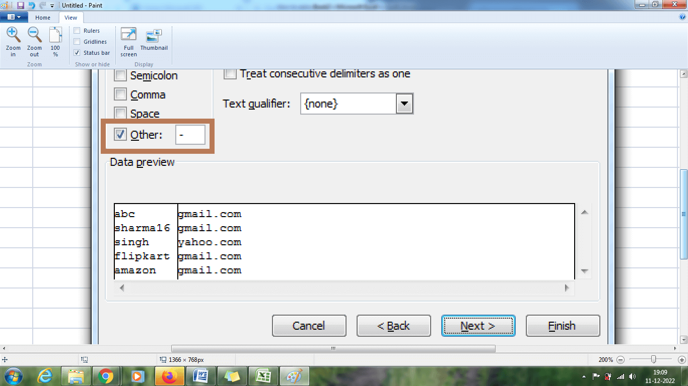
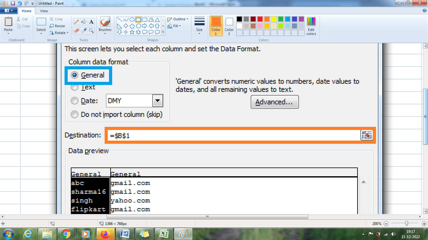
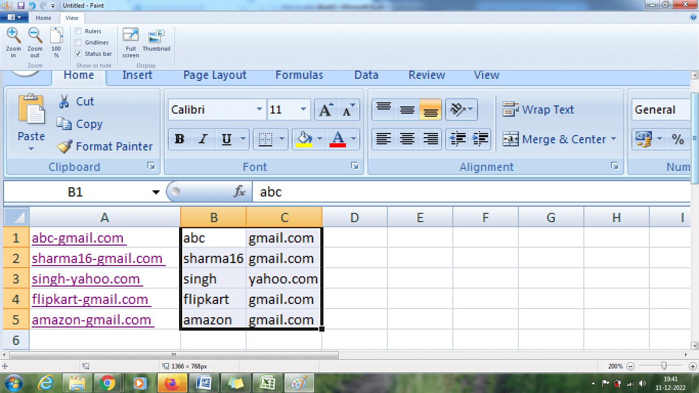
From the above worksheet, the result displayed is Gmail and yahoo without.com. Similarly, this method is followed for other data if the user wishes to display the domain name, as shown in the above method.

Example 6: How to extract the substring using a delimiter in Excel?

Using text functions, the substring is extracted from the given text. If the original text is altered, the result also gets altered where the formula modifies the result based on the data. Here is an alternate method called 'Text to Column' which involves the same process of extracting the substring quickly using markers.

The step to be followed to extract the substring using 'Text to column' is as follows,

1. Enter the required data in the spreadsheet, namely A1:A5. Here in this example, instead of the '@' symbol ',-' is used.
   
2. Select the respective column which contains the data A1:A5. Choose the 'Text to Columns from the Data tools in the Data option.
   
3. The 'text to column wizard' will display. In that, choose the Delimited option in the given option and click 'Next'.
   
4. In 'Convert text to Column Wizard' choose the option 'other' among various options and type the symbol '-'in the box which acts as a delimiter. This delimiter extracts the substring from the given data. Click the option Next.
   
5. Choose the option 'General' among various options and type the Destination cell where the user wants to display the result. Here cell B1 is selected as the destination cell. The data preview shows how the delimiter extracts the substring in the dialogue box. This data preview helps the user to view the result and helps to modify prior if any change is needed. Click Finish.
   
6. The result will be displayed in cell B1:C5. The delimiter displays two substrings in the selected cell, as shown below.
   

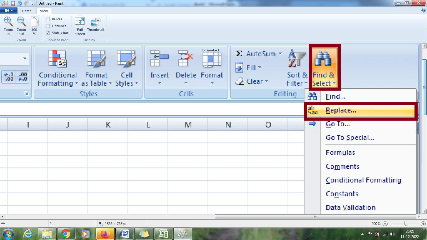
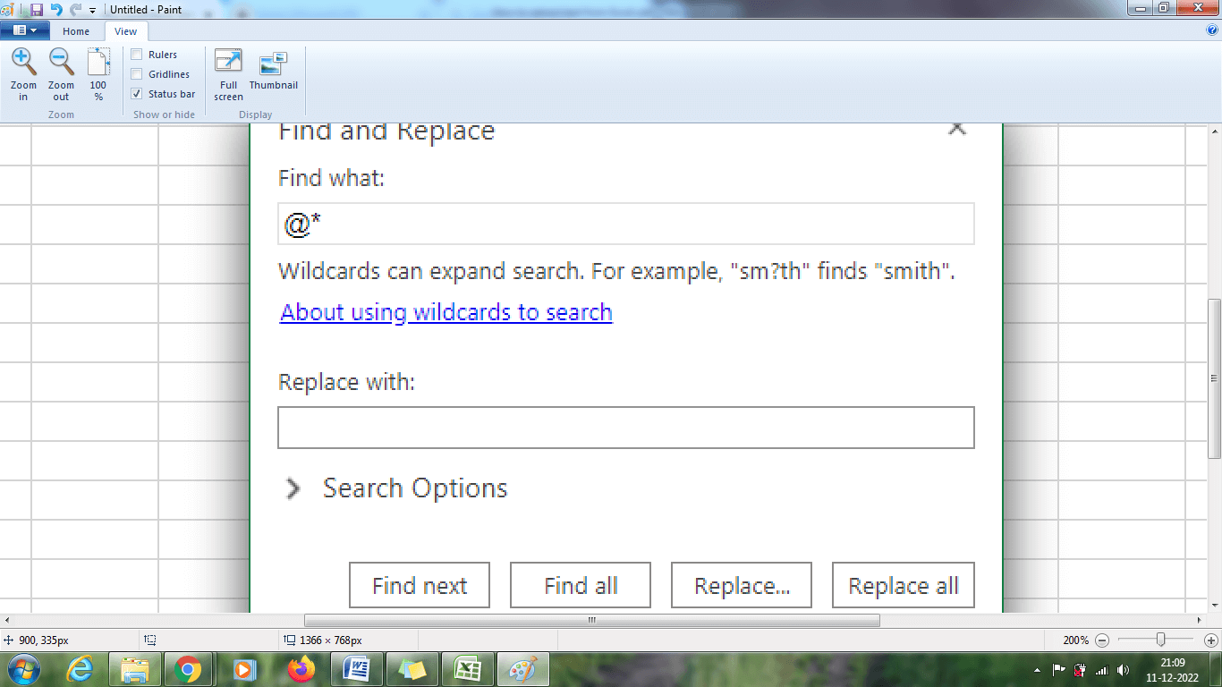
If the user wants to extract the gmail.com to Gmail and .com the same method is repeated to extract the substring from the data.

Example 7: How to use 'Find and Replace' to extract the substring from the data?

Here in this example set of email- IDs are given. The job is to parse the username from the given mail-id. The steps to be followed are,

1. Enter the email-id in the range A1:A5. Copy and paste the data into cell B1:B5. Have a backup of the original data for future reference.
2. Click the Find and Select option in the Home tab from the Editing section. A list of various options will display, and in that, choose the 'Replace' option.
   
3. The Find and Replace dialogue box will display. In that, type @*in, find what box and leave the blank space in Replace with box.
   
4. Click Replace All option. This option removes @gmail.com from the data present in cell A1:A5 and displays only the username.
   

From the above worksheet, only the username is displayed. Here @ an asterisk * is combined to extract the string from the text. An asterisk is a wildcard character which is used to remove the characters. The @ symbol represents the characters counted which are present after it. A @* represents a character that is removed which is present after the @ symbol. Hence the final result will be the username of the given data.

Example 8: How to extract two characters between the parentheses in the data

Sometimes the data are present between slash, brackets, parentheses or braces. To extract the data which is present between the braces, the MID and FIND function is used. The steps to be followed are,

1. Enter the data in the respective cell namely A1:A3.
2. Select a new cell and enter the formula as =MID (A1, FIND ("(", A1) +1, 2). The MID function parses two characters from the data. In the formula, the FIND function finds the position of the opening parenthesis, and the number 1 is added to the starting position of the substring.
3. Press the Enter button. The result will be displayed in the selected cell containing two characters.

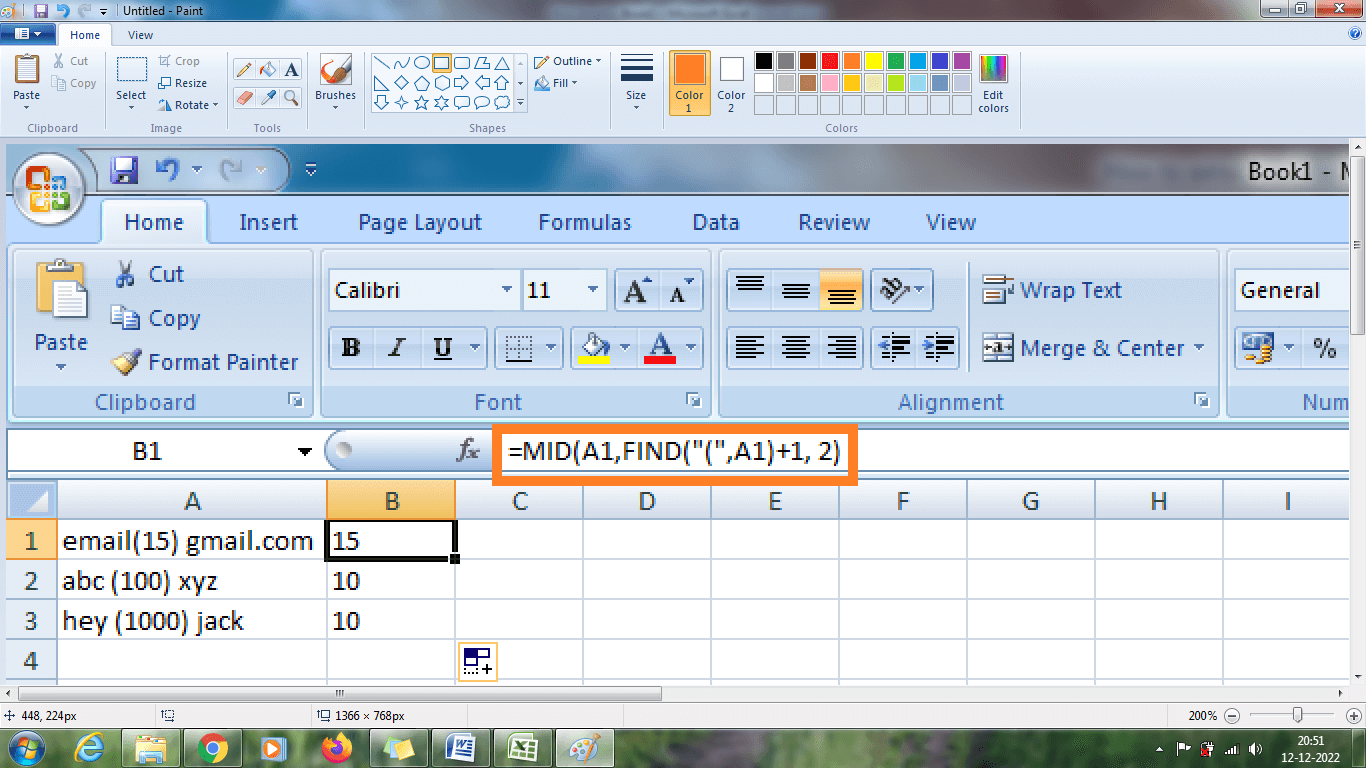
The above worksheet shows the result in column B1:B3, where the MID function extracts two characters from the data. Here for cell A1, the formula will be like =MID (A1, 6+1, 2).Similarly, the same method is followed for all the data in the worksheet.

Example 8.1 How to extract complete characters between the parentheses in the data?

From example 8, only two data are extracted from the data. To extract complete data which is present in the parentheses, the steps to be followed are,

Step 1: Enter the data in the respective cell, namely A1:A3.

Step 2: Select a new cell and enter the formula as =MID (A1, FIND ("(", A1) +1, FIND (")", A1)-FIND ("(", A1)-1). In the formula, the position of the opening parentheses and value one is subtracted from the position of the closing parentheses. The final result will be the position of the substring.

Step 3: Press Enter. The result will be displayed in the selected cell containing two characters.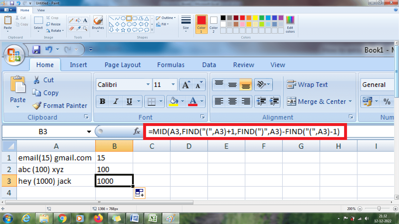

From the above worksheet, the MID and FIND function returns the complete value, which is present between the parentheses.

Example 9: How to extract a selective or specific substring from the given data?

To extract the specific substring from the given data, the steps to be followed are,

1. Enter the data in the respective cell namely A1.
   
2. Select cell A2 and type the formula as =SUBSTITUTE (A1," ", REPT (", 100)). Here SUBSTITUTE and REPT function is used to change the single space with 100 space or the user's preference of space.
   
   The above worksheet mentions the space in the formula as 100. Hence the characters are placed in 100 space distance.
3. To parse the middle present in cell A2, in cell A3, type the formula as =MID (A2, FIND ("@", A2)-50,100). The MID function in the formula generates the middle of the data present in cell A2.
   
4. To remove the space present in cell A3, use the TRIM function. In cell A4, type the formula as =TRIM (A3). The TRIM function removes the space and displays the data, as shown below.
   

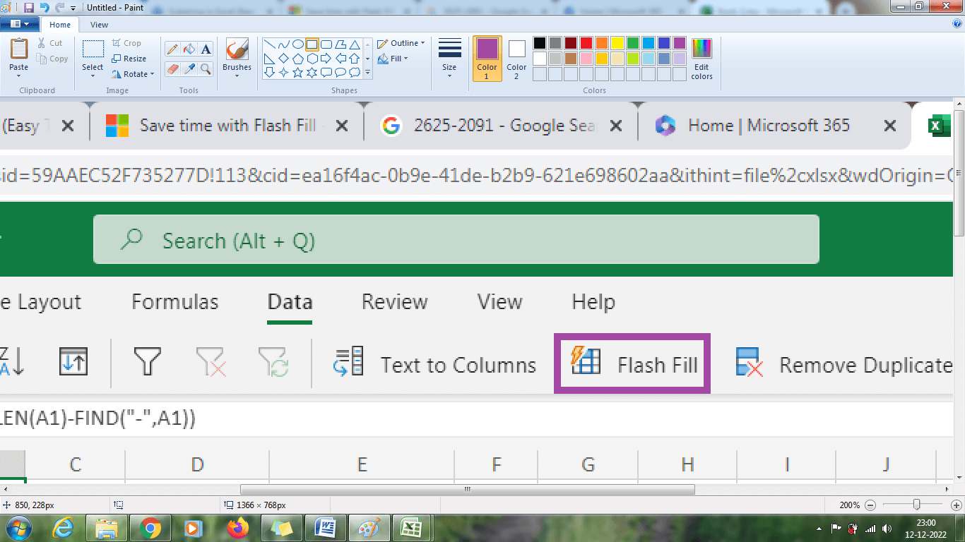
The step-by-step process of extracting the specified or selected substring is explained in step1 to step. To do this method in a single step, the formula is modified as follows,

Flash Fill Method

"A flash-fill method in Excel was used to extract the substring without a formula. It is an alternative and quicker option which parses the string from the given data."

Example 10: How to extract the string from the text using Flash Fill Method?

The steps to be followed to use the Flash Fill method are as follows,

1. Enter the data in the required column A1:A5
2. Enter the parsed data in cell B1. The user must decide the pattern based on extracting the first, second, and last names. Choose the Flash Fill option in the data tab or press CTRL+E. The Flash Fill option automatically updates the pattern in the remaining data.
   
3. The Flash Fill option displays the data in the worksheet below.
   

Example 11: How to use the flash fill method to combine the last name and first name present in the separate column?

In example 10, the flash fill method displays the number pattern. Similarly, to combine the first name and last name, the steps to be followed are,

1. Enter the data in the required column A1:B5.
2. Column A1:A5 contains the last name of the email-id, and B1:B5 consists of the first name of the mail id. To combine and represent the data in a perfect mail-id format, type the format in cell C1 and click the flash fill method. The flash-fill method displays data similar to the data present in C1.
3. The result will be displayed as shown in the worksheet. The pattern present in C1 follows the same pattern up to C5.

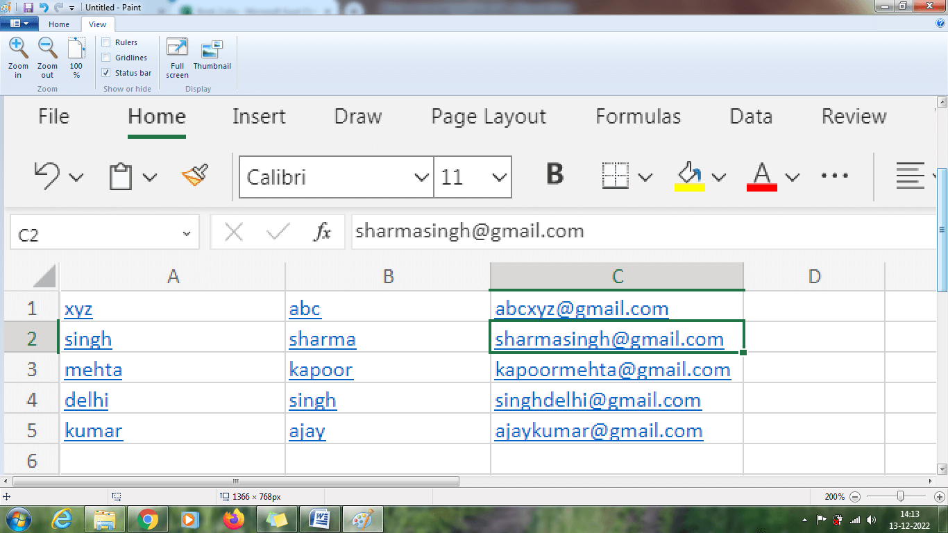
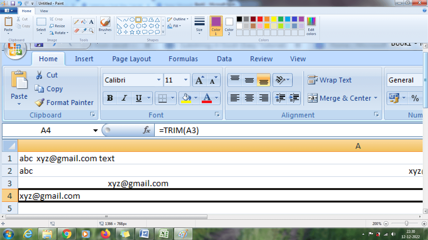
From the above worksheet, the data present in C1:C5 follows the same pattern.

Summary

The above tutorial explains the various methods and functions to extract a substring and text from the data.