How can one remove duplicates in Microsoft Excel?In this modern world, duplicate values in our respective datasheets are very familiar. Still, it could be a big problem, as it can induce substantial errors and overestimate our outcomes. Still, with the help of Microsoft Excel Eliminate Duplicate feature, we can quickly and instantly discover the duplicity's occurrence. We can remove duplicates from rows or from columns efficiently. It is a significant feature of Microsoft Excel, especially when dealing with vast sets of data in which various people put the values in the given datasets respectively. Besides all this, if we want to remove duplicates in Excel from our selected data, then this could be quickly done in Microsoft Excel by just using the various "Methods" which are effectively available. Read this tutorial to learn how to easily find and remove duplicate values from our selected data in Microsoft Excel. Method 1: Removing duplicates from the Excel document So far, removing the duplicates from the Excel sheet, we need to follow the below-mentioned steps very carefully: Step1: Double-click on our Microsoft Excel Document: First of all, we are required to open our computer device and double-click on the Excel Document, and on doing this, we will be navigated to the spreadsheet in Excel. It allows us to open an existing document from the "Recent" option of the open tab respectively. 
Step 2: Select the data: Now after that, from the Excel spreadsheet, we are required to select the data, and for the data selection, we need to click on the top entry of the data and will hold down the Shift key, and click on the bottom entry. If we select multiple columns simultaneously, then we need to click on the top-left entry of the data, then we will click on the bottom-right entry of the data while holding down the Shift key. 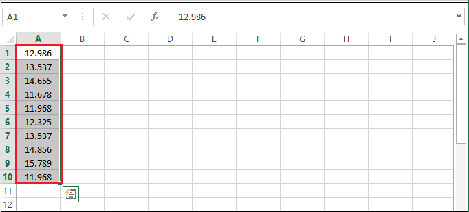
Step 3: Click the Data tab: And once we select the data from the given spreadsheet, we must click on the Data tab, located at the top of theMicrosoft Excel window. 
Step 4: Click Remove Duplicates: And now, after that, we need to click on the Data tab, and a drop-down menu will appear with a list of options where we need to click on the "Remove Duplicates"option. This option is the "Data tools" section of the Data tab, located at the top of the Excel window respectively. 
Step 5: Ensure that each column you want to edit is selected: And if we click on the "Remove Duplicates" option, a pop-up will appear where we must ensure that we have selected each column and want to edit the given spreadsheet. On the given spreadsheet, we will be finding out the various column names, * For example, In column A, Column B, and so on, next to the checkboxes, cling checkboxes will lead to the de-selection of the column, so for this, we need to be careful. And in the Microsoft Excel spreadsheet, all columns next to the one we choose will be listed and checked by default. It allows us to click and Select All to select all the columns listed here. 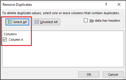
Step 6: Click on Ok when prompted: Now if we click on the "ok " tab, which is located at the bottom right corner of the Remove duplicates windows, a pop-up will appear where we are required to click on the "Ok" tab. Doing this allows us to remove duplicates in our respective Microsoft Excel sheets easily. 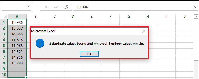
And if no duplicates are shown when we know there are some duplicates, then in that scenario, we need to try and select one column at a time respectively. Method 2: Highlighting of the Duplicates in Microsoft Excel DocumentNow to get a better insight into this method, then we need to follow the below-mentioned steps very carefully: Step 1: Double-click your Excel document: First of all, we are required to open our "computer" and will double-click on the Microsoft Excel document with whom we wish to edit. If we click on the document, it will open the spreadsheet in Excel sheet. And it enables us to check it for the cells consisting of duplicate data values by just using the Conditional Formatting feature of Microsoft Excel. If we wish to look for duplicates but don't want to remove them, then by default, this is a good option for us to do so. And it also enables us to open an existing document for the "Recent" section of the Open tab respectively. 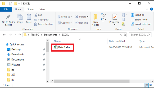
Step 2: Click the top-left cell in your data group: Now after that, once we have selected the document which we wish to edit, then in that case, we are required to click on the top-left cell on the data group; doing so will select it. Here, we must exclude headers from our selection list, such as Day, Date, Time, etc. And if we are going to choose one row, then we need to click on the left-most entry from the data group, and if in case we are going to select one column, then we need to click on the rightmost entry from the data group respectively. 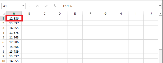
Step 3: Hold on the shift key and click the bottom suitable cell: After now, we need to hold on to the Shift key, and while holding it, we need to click on the bottom suitable cell. It will help us select any data present between the top-left corner and the bottom-right corner of the data group. If we are going to select a single row, then in that case, we need to click on the rightmost cell with a value in it, and if we are going to select a single column, we need to click on the bottom-most entry with a value in it. 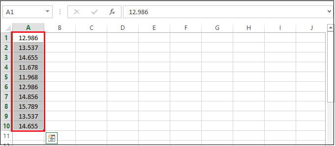
Step 4: Click on the Conditional formatting: Now will be finding out the conditional formatting option in the "Styles" section of the Home page; if we click "Conditional Formatting," a drop-down menu will appear on our screen. After that, we may need to click on the "Home" tabs, which are located near the top of the Excel page, to see this option. 
Step 5: Choose Highlight cells rules From the drop-down menu, we need to select the "Highlight cells rules." A pop-up will appear on our screen once we click on highlight cell rules. 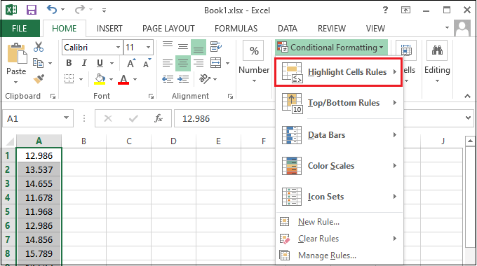
Step 6: Click on the Duplicates value: From the pop-up menu, we must select "Duplicates Values," located at the bottom; doing so will select all duplicate values respectively. 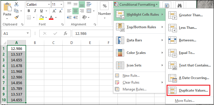
Next TopicHow to advertise on Facebook
|
 For Videos Join Our Youtube Channel: Join Now
Feedback
- Send your Feedback to [email protected]
Help Others, Please Share


