Hyperlink Function in Excel

There is no denying that hyperlink is an important feature of Excel. It helps to directly link a URL to your text. However, Excel provides different methods to create a hyperlink in Excel. To link your text to a specific web page located on Internet, you can simply type its URL in a cell, hit Enter, and Microsoft Excel will automatically convert the entry into a clickable hyperlink. To link the text to another worksheet or specific cell of another workbook, you can use the Hyperlink context menu or press the Ctrl + K shortcut. If you want to add many identical or similar hyperlinks, the easiest method is to use a Hyperlink function, which makes it fast to create, copy and edit hyperlinks in Excel.

In this tutorial, you will learn what is Hyperlink function, its syntax, parameter, points to remember, how this formula works and various examples by using the hyperlink function to link various web pages.

What is a Hyperlink function?

"In Excel, the HYPERLINK function creates a link (shortcut) that directs the user to the given destination or opens another document or web page through a linked text."

The HYPERLINK function in Excel is used to build links to other cells, worksheets, named ranges, workbooks, webpages using the internet, or files available on network servers. The HYPERLINK function can also be used to create email links. This function allows the user to add different types of links in their worksheet depending on what value they want to provide in the link_location parameter.

Using a Hyperlink Excel function, one can link to the below given instances:

• Link any specified location in Excel, i.e., a cell or named range in your worksheet.
• Link to Microsoft Word, Ms PowerPoint, or any other document stored online or on your local network.
• If you want to link the text to a bookmark in a Word document
• To link to different web pages available on the Internet or intranet
• To link text to an Email address so you can compose a new message

The Hyperlink function is an old function and is supported in almost all Excel versions, including Office 365, Excel 2019, Excel 2016, and lower. While using Excel Online, always remember that the HYPERLINK function can only be used for web addresses (URLs).

Syntax

Parameters

Link_location (required): This parameter represents the path to the file or web page (available on the internet) with which you link the text.

Link_location can contain the reference to a cell containing the link, or you can directly refer to the path of a file (text string confined in quotation marks) present on a local drive, UNC path on a server, or URL on the Internet or network server.

NOTE: If the supplied Link_location is wrong or if it does not exist, the Hyperlink function will throw an error.

Friendly_name (optional): This parameter represents the link text to be displayed in a cell present in a worksheet. If this argument is omitted, by default link_location is shown as the link text.

Friendly_name can contain numeric data values, text-based values confined in quotation marks, name, or the reference of a cell that holds the link text.

How to use HYPERLINK in Excel - formula examples

So far, we have covered the theoretical aspects of the HYPERLINK function. Now let's see how we can implement it practically in Excel worksheets. We will cover different examples, including combinations with a few other functions to accomplish a different task.

#Hyperlink Example 1: Using the Excel function hyperlink to another worksheet

The Hyperlink function in Excel allows the user to add different links in their worksheet depending on what value they want to provide in the link_location parameter.

Let's see the step by step process to add a hyperlink to a different worksheet in Excel:

Step 1: Select a target cell

Open your Excel workbook and select a target cell where you want to add the hyperlink to a different sheet. In our case we have selected A2 cell.

Step 2: Insert the hyperlink formula,

• To insert the hyperlink function, start with a '=' sign followed by the Hyperlink function. In its arguments, provide the required Excel sheet name (that you want to link) preceded by a pound sign (#) and followed by the exclamation point and needed cell reference.
• In the next argument, supply the link text to be displayed in a cell present in a worksheet.

Refer to the below formula:

=HYPERLINK("#Sheet2!A1", "Sheet2")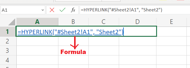

Step 3: Click on the link

Once you are done, click on the enter button. You will notice that a hyperlink with the text 'Sheet2' name will be created.

Refer to the below image: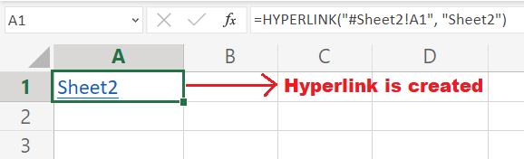

Click on the hyperlink, and to your surprise, the text "Sheet2" will directly jump from sheet1 to Excel to Sheet2 to cell reference A1.

Step 4: Hyperlink to a specific worksheet name

If want to link to a specific worksheet name, don't forget to include the proper spaces or non-alphabetical characters, enclosed between the single quotation symbols.

=HYPERLINK("#'Cash Flow list'!A1", "Cash Flow List")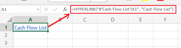

Similarly, you link your cell to another cell reference of the same worksheet in the same workbook. For instance, to add a hyperlink that will direct the user to cell B6 in the same worksheet, use the following formula:

=HYPERLINK("#B6", "Go to cell B6")

#Example 2: Using the Excel Hyperlink link function, link your cell to a different workbook

In the above example, we created the hyperlink of different sheets within the same worksheet. But Microsoft Excel extends the credibility, where you can Hyperlink a cell to another workbook.

Syntax

If you want to hyperlink your cell to another workbook, make sure you supply the full path to the target workbook in the below format:

If you want to hyperlink your cell to a specific sheet even in a specified cell of another workbook, follow the below given format:

To create a hyperlink to another workbook, follow the given below steps:

Step 1: Select a target cell

Open your Excel workbook and select a target cell where you want to add the hyperlink to a different sheet. In our case we have selected A2 cell.

Step 2: Insert the hyperlink formula,

• To insert the hyperlink function, start with a '=' sign followed by the Hyperlink function. In its arguments, provide the source file location (file ending with .xlsx extension) enclosed with double quotes.
• In the next argument, supply the link text to be displayed in a cell present in a worksheet.

Refer to the below formula: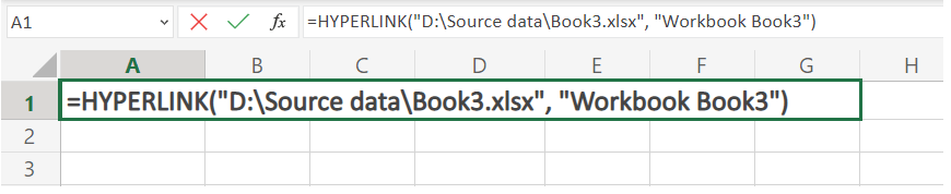

Step 3: Hyperlink to specific sheet of new workbook

To insert a hyperlink titled "Workbook Book3, Sheet2" that will redirect the link to Sheet2 in Book3 located on the Source data folder on drive D, incorporate the following formula: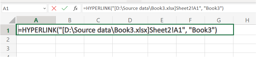

#Example 3: Using Excel Hyperlink function, link the cell to a target named range

To insert a hyperlink to a worksheet-level name, include the full path to the target name in the below format:

To create a hyperlink to worksheet-level name, follow the given below steps:

Step 1: Select a target cell

Open your Excel workbook and select a target cell where you want to add the hyperlink to a different sheet. In our case we have selected A2 cell.

Step 2: Insert the hyperlink formula,

• To insert the hyperlink function, start with a '=' sign followed by the Hyperlink function. In its arguments, provide the link to a range named "Source_data" located on Sheet1 of another workbook Book1 (file ending with .xlsx extension) enclosed with double quotes.
• In the next argument, supply the link text to be displayed in a cell present in a worksheet.

Refer to the below formula:

=HYPERLINK("[D:\Excel files\Book1.xlsx]Sheet1!Source_data","Name Ranged data")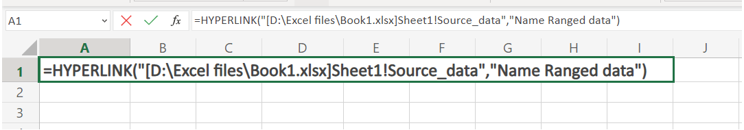

Step 3: Insert hyperlink for workbook-level name

If you are referencing a workbook-level name, the sheet name does not need to be included, for example:

=HYPERLINK("[D:\Excel files\Book1.xlsx]Source_data","Name Ranged Data")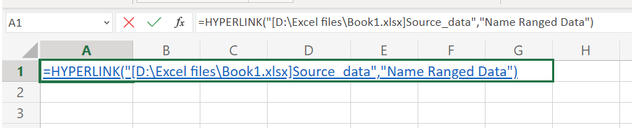

#Example 4: Using the inbuilt hyperlink function, hyperlink to a bookmark in a Word document

To create a hyperlink to a target location in a Word document, confine the document path in [square brackets] and utilize a bookmark to specify the location where you want to redirect the Excel cell.

To create a hyperlink to a specific location in a Word document, follow the given below steps:

Step 1: Select a target cell

Open your Excel workbook and select a target cell where you want to add the hyperlink to a different sheet. In our case we have selected A2 cell.

Step 2: Insert the hyperlink formula,

• To insert the hyperlink function, start with a '=' sign followed by the Hyperlink function. Provide the hyperlink to the bookmark named Subscription_prices in Price list.docx enclosed with double-quotes in its arguments.
• In the next argument, supply the link text to be displayed in a cell present in a worksheet.

Refer to the below formula: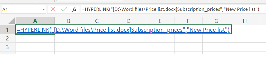

#Example 5: Using the Hyperlink function, link your cell to a web page.

To create a hyperlink to a web-page that is residing on the Internet, provide its URL enclosed within double quotes. Refer to the following format:

To create a hyperlink to a web-page on Internet or Intranet, follow the given below steps:

Step 1: Select a target cell

Open your Excel workbook and select a target cell where you want to add the hyperlink to a different sheet. In our case we have selected A1 cell.

Step 2: Insert the hyperlink formula,

• To insert the hyperlink function, start with a '=' sign followed by the Hyperlink function. In its arguments, provide the URL link of your website enclosed with double quotes.
• In the next argument, supply the link text to be displayed in a cell present in a worksheet.

Refer to the below formula:

=HYPERLINK("https://www.javatpoint.com/","Welcome to JavaTpoint ")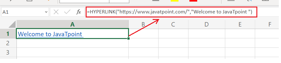

The above formula adds a hyperlink to the title' Welcome to JavaTpoint', which will redirect you to our website's home page.

#Example 6: Using the Hyperlink function, link your cell to send an email

To compose a new message to any recipient, provide an email address in the Hyperlink function in the following format:

To create a hyperlink to send an email, follow the given below steps:

Step 1: Select a target cell

Open your Excel workbook and select a target cell where you want to add the hyperlink to a different sheet. In our case we have selected A1 cell.

Step 2: Insert the hyperlink formula,

• To insert the hyperlink function, start with a '=' sign followed by the Hyperlink function. In its arguments, provide an email address enclosed within the double quotes.
• In the next argument, supply the link text to be displayed in a cell present in a worksheet.

Refer to the below formula: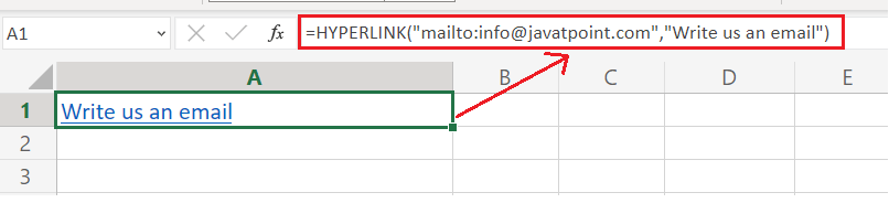

The above formula links the text "Write us an email" to the following Microsoft outlook. Clicking on the link and compose an email to our team.

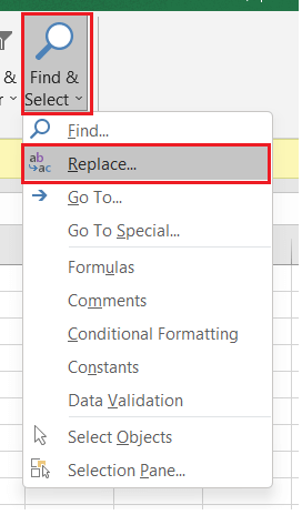
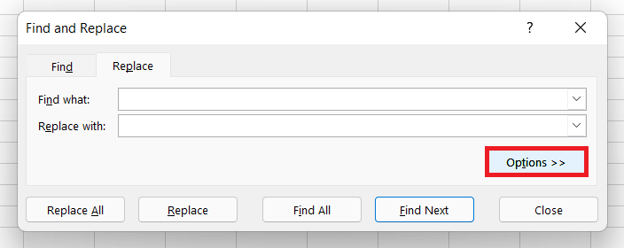
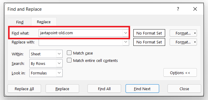
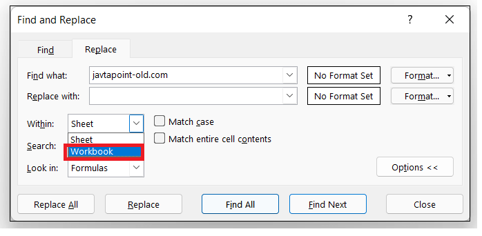
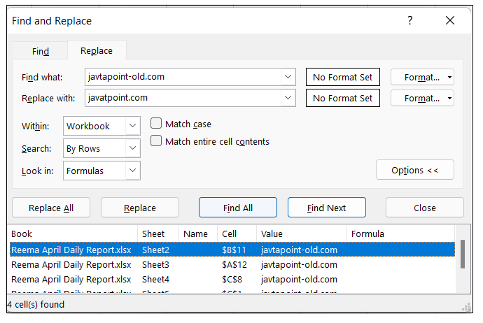
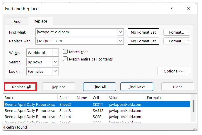
How to edit multiple hyperlinks at a time

One of the most useful advantages of the inbuilt Excel Hyperlink function is its ability to edit multiple Hyperlink formulas at a time by using Excel's Replace All feature. For instance, if you want to replace the old URL of your company with the current one in all hyperlinks on the active.

Follow the below given steps to edit multiple hyperlinks at a time:

1. Open the Replace window (mainly the Find and Replace dialog) either by clicking on Hone->Find & Select-> Replace or by directly pressing the Ctrl + H
   
2. It will open the Find and Replacedialog window. Towards the right side of the window, click the Options button.
   
3. You will have the following window. In the Find whatbox textbox, enter the text you want to change (unlike in our case its "javatpoint-old.com").
   
4. Next, in the 'Within' drop-down window, select either the Sheet or Workbook option as per your requirement. Since we want to change the link for the entire workbook, we have selected the Workbook option.
   
5. In the Look indrop-down list, select the Formulas
6. If you want to be extra precautious, click the Find Allbutton, and as a result, Excel will show all the formulas that contain the search text.
7. In the Replace withbox, type the new text (for instance, in our case its "javatpoint.com").
   
8. Click the Replace All Excel will replace the given text in all found hyperlinks and instantly update you how many replacements it has made.
   
9. That's it, Click the Closebutton to close the Replace window.

Excel HYPERLINK Function not working

Many times while working, we notice that the hyperlinks are not working. In most common cases, the path provided in the link_location argument is broken or is non-existent. If still not resolved, check out the following points:

• While clicking on the hyperlink, if your link destination does not open when you click a hyperlink, please check whether the specified link location is provided in the proper format or not.
• If you received an error unlike VALUE! or N/A while clicking on the link, its because there is some problem with the friendly_name parameter of your Hyperlink function. To prevent these errors, make sure you use the IFERROR functionto show an empty string or some customised instead of the error value.

Eureka! Now you are Hyperlink ready. Go on and create useful hyperlinks using the Excel HYPERLINK function.