| |

Recurrent Neural NetworksWhy not Feedforward Networks?Feedforward networks are used to classify images. Let us understand the concept of a feedforward network with an example given below in which we trained our network for classifying various images of animals. If we feed an image of a cat, it will identify that image and provide a relevant label to that particular image. Similarly, if you feed an image of a dog, it will provide a relevant label to that image a particular image as well. Consider the following diagram: 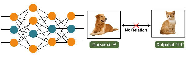
And if you notice the new output that we have got is classifying, a dog has no relation to the previous output that is of a cat, or you can say that the output at the time 't' is independent of output at a time 't-1'. It can be clearly seen that there is no relation between the new output and the previous output. So, we can say that in feedforward networks, the outputs are independent of each other. There are a few scenarios where we will actually need the previous output to get the new output. Let us discuss one such scenario where we will necessitate using the output that has been previously obtained. 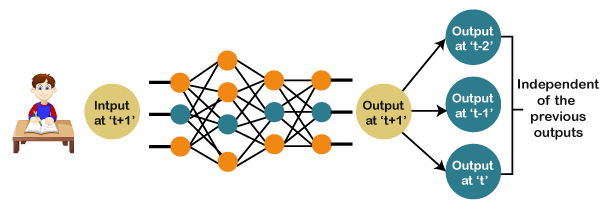
Now, what happens when you read a book. You will understand that book only on the understanding of the previous words. So, if we use a feedforward network and try to predict the next word in the sentence, then in such a case, we will not be able to do that because our output will actually depend on previous outputs. But in the feedforward network, the new output is independent of the previous outputs, i.e., output at 't+1' has no relation with the output at 't-2', 't-1', and 't.' Therefore, it can be concluded that we cannot use feedforward networks for predicting the next word in the sentence. Similarly, many other examples can also be taken where we need the previous output or some information from the previous output, so as to infer the new output. How to overcome this challenge?Consider the following diagram: 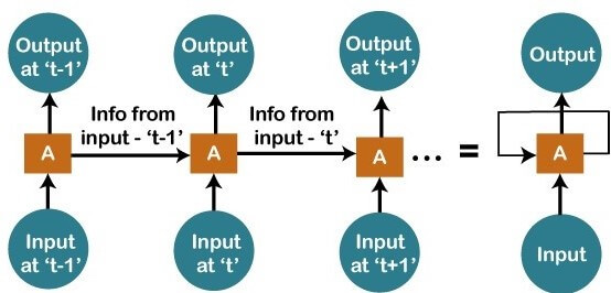
We have input at 't-1', which we will feed to the network, and then we will get the output at 't-1'. Then at the next timestamp that is at a time 't', we have an input at a time 't', which will be again given to the network along with the information from the previous timestamp, i.e., 't-1' and that will further help us to get the output at 't'. Similarly, at the output for 't+1', we have two inputs; one is the new input that we give, and the other is the information coming from the previous timestamps, i.e., 't' in order to get the output at a time 't+1'. In the same way, it will go on further like this. Here we have embodied in a more generalized way to represent it. There is a loop where the information from the previous timestamp is flowing, and this is how we can solve a particular challenge. What are Recurrent Neural Networks?"Recurrent Networks are one such kind of artificial neural network that are mainly intended to identify patterns in data sequences, such as text, genomes, handwriting, the spoken word, numerical times series data emanating from sensors, stock markets, and government agencies". In order to understand the concept of Recurrent Neural Networks, let's consider the following analogy. 
Suppose that your gym trainer has made a schedule for you. The exercises are repeated every third day. The above image includes the order of your exercises; on your very first day, you will be doing shoulders, the second day you will be doing biceps, the third day you will be doing cardio, and all these exercises are repeated in proper order. Let's see what happens if we use a feedforward network for predicting the exercises today. 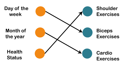
We have provided in the input such as day of the week, the month of the year, and health status. Also, we need to train our model or the network on the basis of the exercises that we have done in the past. After that, there will be a complex voting procedure involved, which will predict the exercises for us, and that procedure won't be that accurate. In that case, whatever output we will get would be as accurate as we want it to be. Now, what if the inputs get changed, and we make the inputs as the exercises that we have done the previous day. 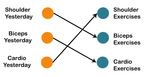
Therefore, if shoulders were done yesterday, then definitely today will be biceps day. Similarly, if biceps were done yesterday, then today will be the cardio day, and if yesterday was the cardio day, then today, we will need to undergo shoulder. Now there can be one such scenario, where you are unable to go to the gym for one day due to some personal reasons, then it that case, we will go one timestamp back and will feed in what exercise happened day before yesterday as shown below. 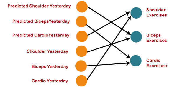
So, if the exercise that happened the day before yesterday was the shoulder, then yesterday there were biceps exercises. Similarly, if biceps happened the day before yesterday, then yesterday would have been cardio exercises, and if cardio would have happened the day before yesterday, then yesterday would have been shoulder exercises. And this prediction for the exercises that happened yesterday will be fed back to our network so that these predictions can be used as inputs in order to predict what exercise will happen today. Similarly, if you have missed your gym say for two days, three days or even one week, you will actually need to roll back, which means that you will need to go to the last day when you went to the gym, you need to figure out what exercises you did on that day and then only you will be getting the relevant output as to what exercises will happen today. Next, we will convert all these things into a vector, which is nothing but a list of numbers. 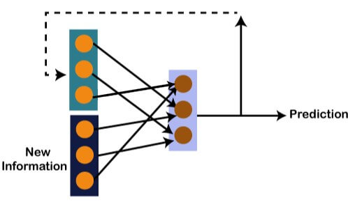
So, there is new information along with the information which we got from the prediction at the previous timestamp because we need all of these in order to get the prediction at a time 't'. Imagine that you did shoulder exercises yesterday, then, in that case, the prediction will be biceps exercise because if the shoulder was done yesterday, then today it will definitely be biceps and output will be 0, 1, and 0, which is actually the work of our vectors. Let's understand the math behind the Recurrent Neural Network by simply having a look at the image given below. 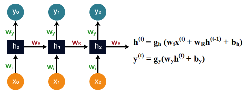
Assume that 'w' is the weight matrix, and 'b' is the bias. Consider at time t=0, our input is 'xo', and we need to figure out what exactly is the 'ho'. We will substitute t=0 in the equation, as shown in the image, so as to procure the function ht value. After that, we will find out the value of 'yo' by using values that were previously calculated when we applied it to the new formula. The same process is repeated again and again through all the timestamps within the model so as to train it. So, this how a Recurrent Neural Networks works. Training a Recurrent Neural NetworkA recurrent neural network uses a backpropagation algorithm for training, but backpropagation happens for every timestamp, which is why it is commonly called as backpropagation through time. With backpropagations, there are certain issues, namely vanishing and exploding gradients, that we will see one by one. Vanishing Gradient Consider the following diagram: 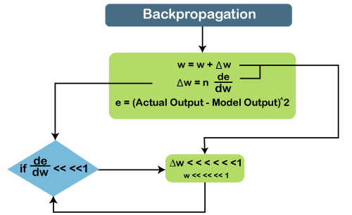
In vanishing gradient when we use backpropagation, we tend to calculate the error which is nothing but the actual output that we already know subtracted by the model output that we got through the model and the square of that, so we can figure out the error, and with the help of that error, we tend to find out the change in error with respect to change in weight or any variable, which is here called as weight. So, the change of error with respect to change in weight multiplied by learning rate will give us the change in rate. And then we will add this change in weight to the old weight to get a new weight. Basically, here we are trying to reduce the error, and for that, we need to figure out what will be the change in error if variables get changed, by which we can get the change in the variable and add it to our old variable to get the new variable. Now over here what can happen if the value de⁄dw, i.e., gradient or simply we can say the rate of change of error with respect to weight variable becomes very smaller than 1 and if we multiply that with the learning rate, which is the definitely smaller than 1, then, in that case, we will get the change in weight, which is negligible. Consider a scenario where you need to predict the next word in the sentence, and your sentence is something like "I have been to USA". Then are a lot of words after that few people speak, and then you need to predict what comes after speak. Now, if you need to do that, then you will have to go back and understand the context of what it is talking about, which is nothing but our long-term dependencies. During the long-term dependencies, de⁄dw becomes very small, and then when you multiply it with n, which is again smaller than 1, you get Δw, which will be very small or simply negligible. So, the new weight that you will get here will be almost equal to your old weight, such that the weight will not get updated further. Also, there will be no learning here, which is nothing but the problem of vanishing gradient. Similarly, if we talk about the exploding gradient, it is actually opposite to that of the vanishing gradient. Consider the below diagram to have a better understanding of it. 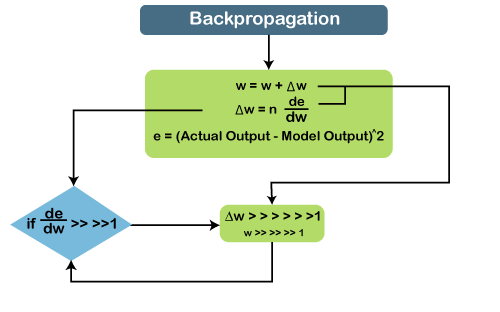
If de⁄dw becomes very large or greater than 1 and we have some long-term dependencies, then, in that case, de⁄dw will keep on increasing, and Δw will become very large that will make the new weight different than that of the old weights. So, these were the two problems with backpropagation, and now we will see how to solve these problems. How to overcome these challenges?
Long Short-Term Memory Networks (LSTMs)Long Short-Term Memory networks, which are commonly known as "LSTMs," are a special kind of Recurrent Neural Networks that are capable enough of learning long-term dependencies. What are long-term dependencies?It has happened many times that we only require recent data in order to perform questions in a model. But at the same time, we may also need data that has been previously obtained. Consider the following example to have a better understanding of it. Let's suppose there is a language model, which is trying to predict the next word on the basis of the previous ones. Assume that we are trying to predict the last word in the sentence say, "The car runs on the road". Here the context is quite simple because the last word always ends up being a road. By incorporating Recurrent Neural Networks, the gap present between the former information and the existing necessities can be easily associated. That is the reason why Vanishing and Exploding Gradient problems do not exist, followed by making this LSTM networks to easily handle long-term dependencies. LSTM encompasses a layer of neural network in the form of a chain. In a standard recurrent neural network, the repeating module consists of one single function as shown in the image given below: 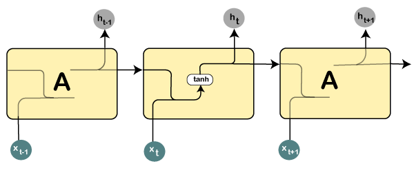
From the image given above, it can be seen that there is a tanh function in the layer, which is called as squashing function. So, what is a squashing function? The squashing function is mainly used in between the range of -1 to +1 so that the values can be manipulated on the basis of inputs. Now, let us consider the structure of an LSTM network: 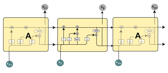
Here all those functions that are present in the layers have their own structures as and when it comes to LSTM networks. The cell state is represented by the horizontal line, acts as a conveyer belt that carries the data linearly crossways the data channel. Let us consider a step-by-step approach to understand LSTM networks better. Step 1: The first step in the LSTM is to identify that information which is not required and will be thrown away from the cell state. This decision is made by a sigmoid layer, which called the forget gate layer. 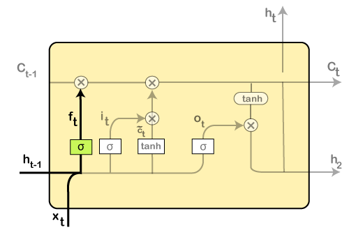
The highlighted layer in the above is the sigmoid layer which is previously mentioned. The calculation is done by considering the new input, and the previous timestamp is, which eventually leads to the output of a number between 0 and 1 for each number in that cell state. As a typical binary, 1 represents to keep the cell state while 0 represents to trash it. ft = σ(wf [ht-1, xt] + bf) where, wf = Weight ht-1 = Output from previous timestamp xt = New input bf = Bias Considering a gender classification problem, it necessitates observing the correct gender when we are using the network. Step 2: Next, we will decide which information we will store in the cell state. It further consists of the following steps:
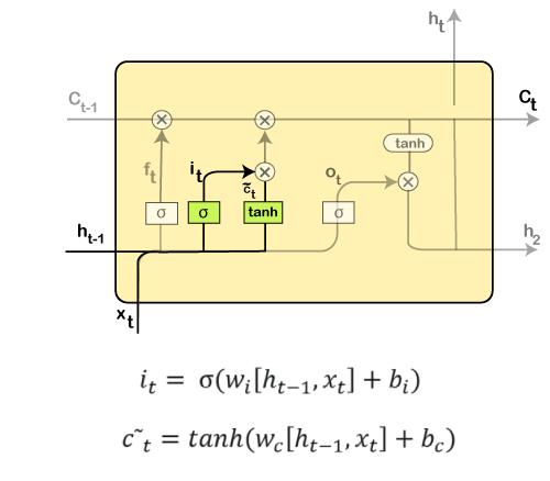
Then the new input, as well as the preceding timestamp's input, will get passed through a sigmoid function that will result in the value i(t), which will then be multiplied by c(t) followed by adding it to the cell state. In the next step, we will combine both of them so as to update the state. Step 3: In the 3rd step, the previous cell state Ct-1 will get updated into the new cell state Ct. And for that, we will need to multiply the old state (Ct-1) by f(t), keeping the things aside that we thought that we earlier decided to leave. 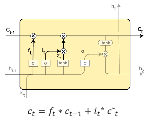
Next, we will add i_t* c˜_t, which is the new candidate values. It has been actually scaled by how much we wanted to update each state value. In the second step, we decided to do make use of the data, which is only required at that stage. However, in the third step, we have executed it. Step 4: In the 4th step, we will run the sigmoid layer that will decide for those parts of the cell state that will result in the output. Next, we will put the cell state through tanh, which means we will be pushing the values in between the range of -1 and 1. And then, further, we will multiply it with the sigmoid gate's output so that only the decided parts results in the output. 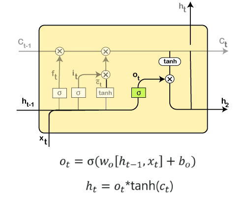
In this step, we will be doing some calculations that will result in the output. However, the output consists of only the outputs there were decided to be carry forwarded in the previous steps and not all the outputs at once. A Quick Recap:
Building an RNNIn this third part of deep learning, which is the Recurrent Neural Networks, we are going to tackle a very challenging problem in this part; we are going to predict the stock price of Google. There is indeed a Brownian Motion that states the future variations of the stock price are independent of the past. So, we will try to predict the upward and downward trends that exist in Google stock price. And to do so, we will implement the LSTM model. We will make an LSTM that will try to capture the downward and the upward trend of the Google stock price because LSTM is the only powerful model that can do this as it performs way better than the traditional models. Apart from this, we are not going to perform a simple LSTM model. It's going to be super robust with some high-dimensionality, several layers as well as it is going to be a stacked LSTM, and then we will add some dropout regularization to avoid overfitting. Also, we will use the most powerful optimizer that we have in the Keras library. In order to approach this problem, we will train our LSTM model on five years of the Google stock price, which is from the beginning of 2012 to the end of 2016 and then based on this training as well as on the identified correlations or captured by the LSTM of the Google stock price, we will try to predict the first month of 2017. We will try to predict January 2017, and again we are not going to predict exactly the stock price, but we are trying to predict the upward and downward trend of the Google stock price. Here we are using the Spyder IDE for the implementation of our RNN model. So, we will start with importing the essential libraries in the 1st part, i.e., data preprocessing followed by importing the training set, and then we will build the RNN. Lastly, we will make predictions and visualize the results. Part1: Data PreprocessingWe will start with, as usual, importing the essential libraries that we will use to implement the RNN just the same way as we did in the earlier model. So, we have NumPy that will allow us to make some arrays, which are the only allowed input of the Neural Networks as opposed to the DataFrames. Then we have matplotlib.pyplot, which we will use to visualize the results in the end. Lastly, the pandas to be able to import the datasets and manage them easily. Output: 
It can be seen in the above image that we have successfully imported these libraries. Next, we will import the training set and not the whole set as opposed to part1 and part2 because we want to highlight that we are going to train our RNN on only the training set. The RNN will have no idea of what is going on in the test set. It will have no acquaintance with the test set during its training. It's like the test set doesn't exist for the RNN. But once the training is done, we will then introduce the test set to the RNN, so that it can make some predictions of the future stock price in January 2017. This is why we are only importing the training set now, and after the training is done, we will import the test set. So, to import the training set, we will first need to import the data as DataFrames, which we will import with pandas using the read_csv function. But then remember we have to not only select the right column that we need, which is the open Google stock price, but also, we need to make it a NumPy array because only the NumPy array can be the inputs of neural network in Keras. Output: 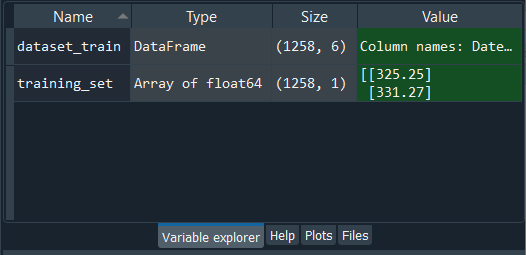
From the above image, we can see that dataset_train is the DataFrame and training_set is the NumPy array of 1258 lines corresponding to 1258 stock prices in between 2012 and 2016, and one column, which is the open Google stock price. We can open them by clicking on the dataset_train and training_set one by one. 
Now we can precisely check from the above image that the open Google stock price in training set with the same number of lines, i.e., the same number of stock prices. So, we have a NumPy array of one column but not the vector. After this, we will apply the feature scaling to our data to optimize the training process, and feature scaling can be done in two different ways, i.e., standardization and normalization. In standardization, we subtract the observation by the mean of all observations in one same column and then divide it by the standard deviation. However, in normalization, we subtract the observation by the minimum of all observations, i.e., the minimum stock prices, and then we divide it by the maximum of all the stock prices minus the minimum of all the stock prices. So, this time is more relevant to use normalization because whenever we build an RNN and especially if there is a sigmoid function as the activation function in the output layer of the recurrent neural network, it is recommended to apply normalization. Therefore, we will apply normalization, and to do this, we will import the min-max k-load class from the preprocessing module of the scikit learn library, and then from this preprocessing module, we will import the MinMaxScaler class. Now from this class, we will create an object of the same class, which we will call as sc for scale. And sc will be the object of MinMaxScaler class inside of which we will pass the default argument, i.e., feature_range. Here we have made feature_range equals to (0, 1) because if we look at the case of normalization, we will see that all the new scaled stock processes will be between 0 and 1, which is exactly what we want. Next, we will apply the sc object on our data to effectively apply the normalization. For this we will introduce a new variable which will be the scaled training set, so we will name it as training_set_scaled, and in order to get the normalized training set, we will simply take the sc object followed by applying fit_transform method, which is the method of MinMaxScaler class so as to fit the sc object to the training_set that we will input as an argument and then scale it. Basically, fit means that it is just going to get the min of the data, i.e., the minimum stock price and the maximum stock price to be able to the normalization formula. And then, with the transform method, it will compute for each of the stock prices of the training set, the scaled stock prices according to the formula. Output: 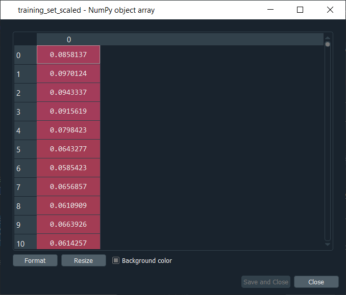
After executing the above lines of code, we will obtain our training_set_scaled, as shown in the above image. And if we have a look at it, we can see that indeed all the stock prices are now normalized between 0 and 1. In the next step, we will create a specific data structure, which is the most important step of data preprocessing for Recurrent Neural Networks. Basically, we are going to create a data structure specifying what the RNN will need to remember when predicting the next stock price, which is actually called the number of timesteps and it is very important to have a right number of timesteps because the wrong number of timesteps could lead to overfitting or baseless predictions. So, we will be creating 60 timesteps and 1 output, such that 60 timesteps mean that at each time T, the RNN is going to look back at 60 stock prices before time T, i.e., the stock prices between 60 days before time T and time T, and based on the trends, it is capturing during these 60 previous timesteps, it will try to predict the next output. So, 60 timesteps of the past information from which our RNN is going to learn and understand some correlations or some trends, and based on its understanding, it's going to try to predict the next output, i.e., the stock price at time t+1. Also, 60 timesteps refer to 60 previous financial days, and since there are 20 financial days in one month, so 60 timesteps correspond to three months, which means that each day we are going to look at the three previous months to try to predict the stock price the next day. So, the first thing that we need to create two separate entities; the first entity that we will create is X_train, which will be the inputs of the neural network, and the second will be y_train that will contain the output. Basically, for each observation, or we can say for each financial day, X_train will contain 60 previous stock prices before that financial day, and y_train contain the stock price of the next financial day. We will start initializing these two separate entities, i.e., X_train and y_train, as an empty list. The next step is for a loop because we will populate these entities with 60 previous stock prices in X_train and the next stock price in the y_train. So, we will start the loop with 60 because then for each i which is the index of the stock price observation, we will get the range from i-60 to i, which exactly contains the 60 previous stock prices before the stock price at time t. Therefore, we will start the range at 60 because then the upper bound is much easier to find, which is off course, the last index of our observation, i.e., 1258. Inside the for loop, we will start with X_train, which is presently an empty list, so we will append some elements into the X_train by using the append function. We will append the 60 previous stock prices before the stock price at index i, i.e., the stock price at the ith financial day. So, in order to get them, we will get our training_set_scaled, and in this, we will take 60 previous stock prices before the ith financial day, which is the range of the indexes from i-60 to i. Since we already selected correct lines for X_train, but we still need to specify the column and as we have one column in the scaled training set, i.e., the column of index 0, which is exactly what we need to add here. Now, in the same way, we will do for y_train, which will be much easier because we simply need to input the stock price at time t+1, and therefore we just need to do the same here. The stock price at t+1 is, of course, going to be taken from training_set_scaled and inside it we will take same indexes for columns, i.e., 0, but for the observation line, we will take the ith index because if we consider the same example when we have i equal to 60, then X_train will contain all the stock prices from 0 to 59 as the upper bound was excluded, but what we want to predict is actually based on the 60 previous stock prices is the stock price at time t+1, which is 60 and that is the reason we input i here instead of i+1. So, now we have the 60 previous stock prices in X_train and the stock price at time t+1 in y_train. Since X_trian and y_train are lists, so we again need to make them NumPy arrays for them to be accepted by our future Recurrent Neural Network. Output: Once we execute the above give code, we can have a look at X_train and y_train by clicking them individually on the from the variable explorer pane. X_train 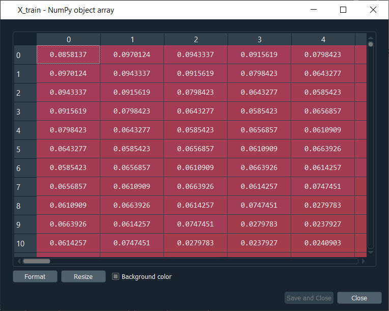
As we can see from the above image, X_train is a special data structure. Here the first line of observation corresponds to time t equals 60, which means it corresponds to the stock price at the 60th financial day of our training dataset. And all those values are the previous 60 stock prices before that stock price at the 60th financial day, which means that there are 59 values here, such that if we have a look at the first line, i.e., observation of the 1st index, corresponds to the stock price at the 61st financial day of the training set. All these stock prices are the preview stock prices before that 61st stock price of our training dataset. y_train 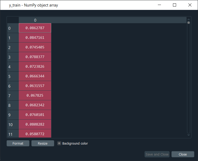
Now if we have a look at y_train, we can see it very simple to visualize as it contains the stock price at time t+1 and if compare both the X_train and y_train, we will see that X_train contains all the 60 previous stock prices t = 60, and based on the stock prices of each individual line, we will train our Recurrent Neural Network to predict the stock price at time t+1. After this, we will perform our last step of data pre-processing, which is reshaping the data, or in simple words, we can say we will add some more dimensionality to the previous data structure. And the dimensionality that we are going to add is the 'unit', i.e., the number of predictors that we can use to predict the Google stock prices at time t+1. So, in the scope of this financial engineering problem where we are trying to predict the trend of the Google stock price, these predictors are indicators. Presently we are having one indicator, which is the Google Stock Prices and so we are taking 60 previous Google stock prices to predict the next one. But with the help of a new dimension that we are going to add to our data structure, we will be able to add some more indicators that will help in predicting even better the upward and downward trends of the Google Stock Price. We will use the reshape function to add a dimension in the NumPy array. We just need to do this for X_train because it actually contains the inputs of the neural network. So, we create a new dimensionality of the new data structure because simply that is exactly what is expected by the future recurrent neural network that we are going to build in our 2nd part. So, we will start by updating the X_train by using the reshape function, which is taken from the NumPy library because we are reshaping a NumPy array. Inside the reshape function, we will input the following arguments:
Output: 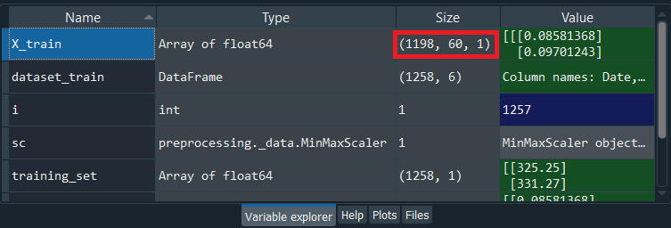
By executing the above line of code, we will see that we have our new X_train, and if we have a look at the above image, we will see that it has the three dimensions, the exact same ones as we just mentioned. Further to have a look at X_train, we will need to again click on it from the Variable explorer pane, and it will be like something as given below. 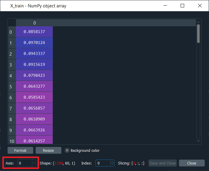
From the above image, we can clearly visualize that although it is not in the 3-dimension, so we can see it simply by changing the axis. As we can see in the image, it is in the 1-dimension, the axis is 0. In the same way, we will see the rest of the axis that corresponds to the three dimensions of the structure. Now that we are done with the data preprocessing, we will now move on to part2, i.e., building the Recurrent Neural Network, where we will build the whole architecture of our stacked LSTM with several LSTM layers. Part 2 - Building the RNNIn the second part, we are going to build the whole architecture of the neural network, a robust architecture, because we are not only going to make a simple LSTM but a stacked LSTM with some dropout regularization to prevent overfitting. So, we will not import the Sequential class that will help us in creating the neural network object representing a sequence of layers, but also the Dense class to add the output layer. We will also import the LSTM class to add the LSTM layers and then the Dropout class to add some dropout regularization. This is all that we need to build a powerful RNN. Output: 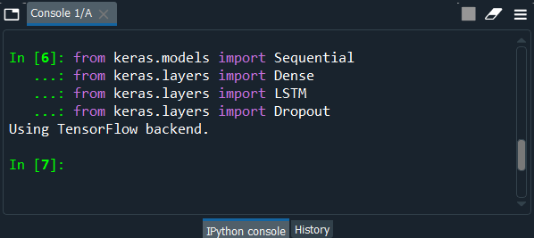
Using the TensorFlow backend, all the classes are imported, as shown above. Next, we will initialize our Recurrent Neural Network as a sequence of layers as opposed to a computational graph. We will use the Sequential class from the Keras to introduce the regressor as a sequence of layers. Regressor is nothing but an object of the sequential class that represents the exact sequence of the layers. We are calling it as regressor as opposed to the classifiers in ANN and CNN models because this time, we are predicting a continuous output, or we can say a continuous value, which is the Google stock price at time t+1. So, we can say that we are doing a regression, which is all about predicting continuous value, whereas classification was predicting a category or a class, and since we are predicting a continuous value, this is the reason why we called our Recurrent Neural Network a regressor. After initializing the regressor, we will add different layers to make it a powerful stacked LSTM. So, we will start by adding the first LSTM layer of our Recurrent Neural Network, which was introduced as a sequence of layers and also some dropout regularization so as to avoid overfitting as we don't want while predicting the stock price. We will do this in two steps: we will add the first LSTM layer, and then we will add the dropout regularization. Let's starts with adding our first LSTM layer, and for that, we will take our regressor, which is an object of the sequential class. The sequential class contains the add method that allows adding some layers of the neural network, and inside the add method, we will input the type of layer that we want to add, i.e., an LSTM layer and that is where we use the LSTM class because actually what we are adding in this add method will be an object of the LSTM class. Therefore, we create the LSTM layer by creating an object of the LSTM class, which will take several arguments that are as follows:
After we are done with our first step, now we will take care of the second sub-step of the first step building the architecture of the neural network, i.e., adding some Dropout regularization and to do this, we will again take our regressor followed by using the add method of the sequential class because it will work the same way as for the LSTM. We will start by creating an object of the Dropout class that we already imported to include this dropout regularization. Therefore, exactly as for LSTM, we need to specify here the name of this class as Dropout that will take only one argument, i.e., Dropout rate, which is nothing but the number of neurons that we want to drop or in simple words that we want to ignore in the layer to do this regularization. And the relevant number to use them is to drop 20% of the neurons in the layer, which is exactly that we need to input here. This is the reason why we have added 0.2 as it corresponds to 20%. So, we will 20% of dropout, i.e., 20% of the neurons of the LSTM layer will be ignored during the training that is during forward and backward propagation happening in each iteration of training. Therefore, since 20% of 50 is 10 neurons, which simply means that 10 neurons will be ignored and dropped out during each iteration of the training. Hence, we are done here with our first LSTM layer, to which we added some dropout regularization. Now we will add some extra LSTM layers followed by adding to each of them some dropout regularization. So, we will start by adding our second LSTM layer in the same way as we did in the previous step because we will again use the add method from the sequential class to add a new LSTM layer and some dropout regularization to our regressor, but we will do some changes to the input_shape argument. As in the previous step had to specify the input_shape argument because that was our first LSTM layer and we were required to specify the shape of the input with the last two dimensions corresponding to the timesteps and the predictors, but now things are slightly different, we are just adding our second LSTM layer, which is why we don't need to specify it anymore. Since it is automatically recognized, so will skip adding it to the code when we are adding our next LSTM layers after the first one. Therefore, we will keep the same number of neurons in the second LSTM layer, i.e., 50 neurons, as well as the same 20% dropout for the regularization due to the fact that it's a relevant choice. Similarly, in order to add our third LSTM layer, we will exactly copy the above two lines of code that added out the second LSTM layer because adding the third LSTM layer is similar to that of adding the second LSTM layer. We simply need to specify the number of neurons in the LSTM layer, which we are keeping it as 50 neurons so as to have the same goal of having a high dimensionality. We still need to keep return_sequences equal to True because we are adding another LSTM layer after the second LSTM layer, and again, we will keep 20% dropout regularization. Next, we will add our fourth LSTM layer, but this time things will be slightly changed. We will keep 50 neurons in this fourth LSTM layer because this is not the final layer of the Recurrent Neural layer. But after the fourth layer, we will have our output layer with the output dimension, which will be 1, of course, as we are predicting only one value, the value of the stock price at time t+1. Since we are adding the fourth LSTM layer, which is the last LSTM layer that we are adding, so we will need to set the return_sequences equal to False because we are not going to return any more sequences. But as we know, the default value for the return_sequences parameter is False, so we will just remove that part as that is what we have to do for the fourth LSTM layer. We are just adding the LSTM class with 50 units, and the same we will keep the 20% dropout regularization. Output: 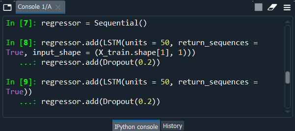
From the above image, we can clearly see that we are successfully done with the LSTM part. Now we just need to add our final layer, which is the output layer. We will simply take our regressor, which is exactly the same as for the ANN and CNN, followed by adding the add method again from sequential class to add the final output layer of our neural network. Since we are not adding the LSTM layer, but actually a classic fully connected layer because the output layer is fully connected to the previous LSTM layer, so in that case to make it a fully connected layer, we will need to use the Dense class exactly as we did for the ANN and CNN. So, we will specify the Dense class in the add method, and then we will add one argument which will correspond to the number of neurons that are needed to be in the output layer. Since we are predicting a real value corresponding to the stock price, so the output has only one dimension, which is exactly what we need to input and the argument for that is units as it corresponds to the number of neurons in the output layer or the dimension of the output layer, which is 1. Now that we are done with the architecture of our super robust LSTM recurrent neural network, we have two remaining steps of Building the RNN; first one is compiling the RNN with a powerful optimizer and the right loss, which will be the mean squared error because we are doing some regression and the second step is to fit this recurrent neural network to the training set. Since our training set is composed of X_train, which is the right data structure expected by the neural networks, so we will take X_train instead of the training set or the training_set_scaled, and of course, we will need to specify the outputs when fitting the regressor to our training sets because the output contains the ground truth that is the stock price at time t+1. As we are training the RNN on the truth, i.e., the true stock price that is happening at time t+1 after the 60 produced stock prices during the 60 produced financial days, so that's why we also need to include the ground truth, i.e., y_train. Let's compile the RNN with the right optimizer and the right loss function. So, we will start by taking our regressor as we are predicting a continuous value followed by using the compile method, which is another method of a sequential class, and inside the compile method, we will input two arguments, i.e., the optimizer and the loss function. In general, for recurrent neural network, an RMS prop optimizer is recommended, but in our case of a problem, we will be using adam optimizer because it's always a safe choice as it very powerful and always perform some relevant updates of the weights. And the second argument that we will input is the loss function. Since we are not dealing with the classification problem, but the regression problem because we have to predict a continuous value, so this time the loss function is mean_squared_error due to the fact that the error can be measured by the mean of the squared differences between the predictions and targets, i.e., the real values. After compiling the RNN, we will fit the RNN to the training set that is composed of X_train and y_train. So, we will again start by taking the regressor and not the classifier followed by using the fit method, which will not only connect the neural network to the training set but will also execute the training over a certain number of epochs that we will choose in the same fit method. Inside the fit method, we will pass four arguments that are the X_train, y_train, epochs, and the batch_size. So, our network is going to be trained not on the single observation going to the neural network but on the batches of observation, i.e., the batches of the stock prices going into the neural network. Instead of updating the weights every stock price being forward propagated into the neural network and then generating an error, which is backpropagated into the neural network, we will do that for every 32 stock prices because we have chosen the batch_size of 32. So, here we are done with building a super robust recurrent neural network as well as we are ready to train it on 5 years of the Google Stock Prices. Output: 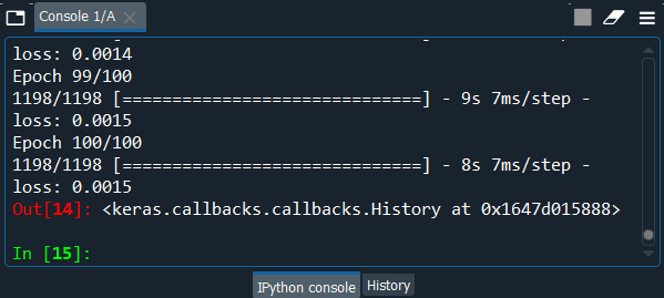
From the above image, we can see that we have prevented enough the overfitting to not decrease the loss even more because if we had obtained too small loss in the end, we might have got some overfitting, as well as our predictions, will be closed to the real Google stock price. In the training data, which is the data of the past but not the one in which we are interested in making predictions, we will get some great loss on it and some really bad loss on the test data. So, this is exactly what overfitting is all about. This is the only reason when we train the training set, we must be careful not to obtain overfitting and therefore not to try to decrease the loss as much as possible, which is why it seems that we get really good results. After this, we will move on to the 3rd part in which we will visualize our predictions compared to the real Google stock price of the first financial month of 2017. # Part 3 - Making the predictions and visualizing the resultsFirst, we will get the real stock price of 2017, then in the second step, we will get the predicted stock price of 2017, and lastly, we will visualize the results. So, in order to get the real stock price of 2017, we will get it from the test set in the CSV file, and therefore we will just do exactly the same as what we did for our training set. We will simply start with creating a data frame by importing the Google_Stock_Price_Test.csv file with the read_csv function by pandas, and then we will select the right column, the open google stock price followed by making it a NumPy array that we will do by replacing the training set by the test set. Since the test set is going to be the real values of the Google stock price in the first month of After executing the above code, we will have the real_stock_price of January 2017 and we can have a look at it in the variable explorer pane. Output: 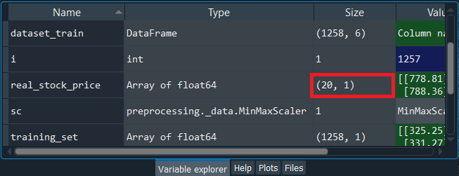
From the above image, we can see that the real_stock_price comprises 20 observations, i.e., 20 stock prices, because these are financial days, and there are 20 financial days in one month, excluding Saturdays and Sundays. We can have a look at it by clicking on real_stock_price, and it will be like something as given below. 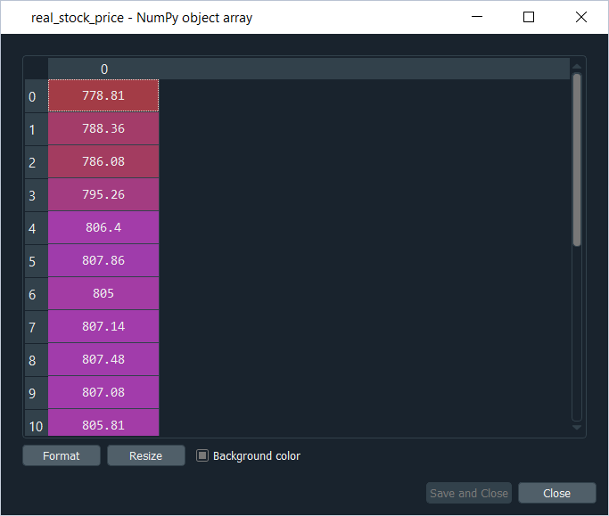
Next, we will move onto our second step in which we will the predicted stock price of January 2017. So, here we will use our regressor with the help of which we are going to predict the Google stock prices of January 2017. Basically, the first key point is that we trained our model to predict the stock price at time t+1 based on the 60 previous stock prices and therefore to predict each stock price of each financial day of January 2017, we will need the 60 previous stock prices of 60 previous financial days before the actual day. Then the second key point is, in order to get at each day of January 2017, the 60 previous stock prices of the 60 previous days, we will need both the training set as well as the test set because we will have some of the 60 days that will be from the training set as they we will be from December 2016, and we will also have some stock prices of the test set due to the fact that some of them will come from January 2017. Therefore, the first thing that we need to do is some concatenation of the training set and the test set to be able to get these 60 previous inputs for each day of January 2017, which then leads to understanding the third key point. We will be making this concatenation by concatenating the training set and the test set, i.e., by concatenating the training set that contains the real Google stock prices from 2012 to the end of 2016, such that is concatenated this training set with the test set will actually lead to a problem because then we will have to scale this concatenation of the training set and the test set. To do that, we will have to apply the fit_transform method from the sc object that we created in the feature scaling section to scale the concatenation of the training set and the test set to get the scaled real_stock_price. But it will change the actual test values, and we should never do this, so we will keep the actual test values as they are. Therefore, we will make another concatenation, which will be to concatenate the original DataFrames that we still have, i.e., dataset_train and dataset_test and from this concatenation, we will get the inputs of each prediction, which is the produced stock prices at each time t and this is what we will scale. These are those inputs that we will apply on our sc object as well as scale to get the predictions. In this way, we are only scaling the input instead of changing the actual test values and will lead us to the most relevant results. So, we will start by introducing a new variable called dataset_total as it will contain the whole dataset, and then we will do concatenation for which we will use the concat function from the pandas library. Inside the pandas function, we need to input two arguments such as the first one is the pair of two DataFrames that we want to concatenate, i.e., we will concatenate the dataset_train to the dataset_test, and the other argument is the axis along which we want to make this concatenation. Since we want to make this concatenation along lines as we want to add the stock prices of the test set to that of the training set, so we will make the concatenation along the vertical axis and to specify this we will add the second argument, i.e., axis=0 because the vertical axis is labeled by 0. Now in the next step, we will get the inputs, i.e., at each time t or each financial day of January 2017, we need to get the 60 previous stock prices of the 60 previous financial days. So, to get these inputs, we will start by introducing new variable inputs. Then we will get the dataset_total because we are getting these stock prices from our DataFrame, dataset by so far, and therefore as we will need the stock prices from the first financial day of 2017 minus 60, up to the last stock price of our whole dataset. For that, we get our first lower bound of this range of inputs that we need. The lower bound is the stock price at January 3rd minus 60 and to get that we will need to find the index of January 3rd, which will simply do by taking len(dataset_total), which is the length of the total dataset followed by subtracting it to the len(dataset_test), which is the length of the dataset and as we want to get the stock price at this day, so we will see again minus it by 60 because it is the lower bound of the inputs that we require. And to get the upper bound, we will simply need to add a colon (i.e. :). Basically, the upper bound is the last index of the whole dataset because to predict the last stock price of the last financial day, we will need the 60 previous stock prices, and therefore the last stock prices we will need is the stock price just before that last financial day. So, this is the range of inputs that will result in the DataFrame, but of course, we need to move on to NumPy arrays, and for that, we will add dot values to make it a NumPy array. All of these will contain all the inputs that we will need to predict the stock prices of January 2017. In the next step, we will make the simple reshape to get the right NumPy shape, so we will update the inputs, and to do that, we will again take the same old inputs that we took in the previous step to which we will further add the reshape function. Inside the reshape function, we will pass (-1, 1) as it will help us to get inputs with different stock prices of January 3rd - 3 months up to the final stock prices in lines and in 1 column. Now we will repeat the same process that we did before also to obtain the right 3D format, which is expected by the neural network not only for training but for the predictions too. So, whether we apply the fit method to train the regressor or to predict method to make the regressor predict something and for that, we need to have the right format of inputs, which is the 3D format that we made previously. Before starting with making this 3D special structure, we have to scale our inputs because they are directly coming from the original DataFrames contained in dataset_total, so we have the original values of the stock prices and since our recurrent neural network was trained on the scaled values, well, of course, we need to scale the inputs, which satisfies here the 3rd key point that we discussed earlier, i.e., to scale the inputs only and not the actual test values because we need to keep the test values as it is. So, we will start by updating the inputs again for which we will the scaling object, which is sc, but here we will not use the fit_transform method because the sc object is already fitted to the training set due to which we will directly use the transform method as the scaling we need to apply to our input must be the same scaling that we applied to the training set. Therefore, we must not fit our scaling object sc again, but we must directly apply the transform method to get the previous scaling on which our regressor was trained Next, we will create a special data set structure for the test set, so we will introduce a new variable and call it as X_test because it will be the input that we will need to predict the value of the test set. Since we are not doing any training, so we would need the y_test. We are actually doing some predictions, so we don't need a ground truth anymore, which is why y_train is also not included here and inside the loop, we will not change the lower bound to get 60 previous time steps, and since we are i-60 here, so we must start at 60. But then for the upper bound, things are quite different because all that we are doing is to get the input for the test set as it contains only 20 financial days, so we need to go up to 60+20=80, and with this, we will get our 60 previous inputs for each of the stock prices of January 2017 that contains 20 financial days. After this we will append in X_test, the previous stock prices, which are indeed taken from the inputs and keep its range of the indexes from i-60 to i, we are also keeping 0 as it corresponds to the Open Google Stock Prices and anyway there is only one column in the inputs. Since X_test is also a list, so we again need to make it a NumPy array so that it can be accepted by our future Recurrent Neural Network and by doing this we have a structure where we have in each line of observations, i.e., for each stock prices of January 2017, we have in 60 columns the 60 previous stock prices that we need to predict the next stock price. Now we will further move on to get the 3D format for which we will again use the reshape function to add a dimension in NumPy array. We will do in the exact same way as we did in the reshaping section of Data preprocessing part, just we need to replace X_train by X_test and the rest code as well as its explanation is similar as discussed above. So, we are ready to make predictions as we have right 3D structure of our inputs contained in X_test, which is exactly what is expecting our recurrent neural network regressor and therefore we are ready to apply our predict method from this regressor to get our predicted stock prices of January 2017. We are going to take the regressor, and from this regressor, we will apply the predict method to which we need to input the X_test that contains the inputs in the right format to predict the stock prices of January 2017. Since it returns predictions, so we will store these predictions in a new variable named as predicted_stock_price that will be consistent with the real_stock_price followed by making it equal to what is returned by the predict method taken from our regressor and apply it to the right input contained in the X_test. After doing this, we will inverse the scaling of our predictions because our regressor was trained to predict the scaled values of the stock price, so in order to get the original scale of these scaled predicted values, we simply need to apply the inverse_transform method from our scaling sc object. Since we are going to update the predicted_stock_price with the right scale of our Google stock price values, so we will get our predicted_stock_price followed by taking our scaling object, i.e., sc and that's where we will apply the inverse_transform method to which we are going to apply the predicted_stock_price. Output: 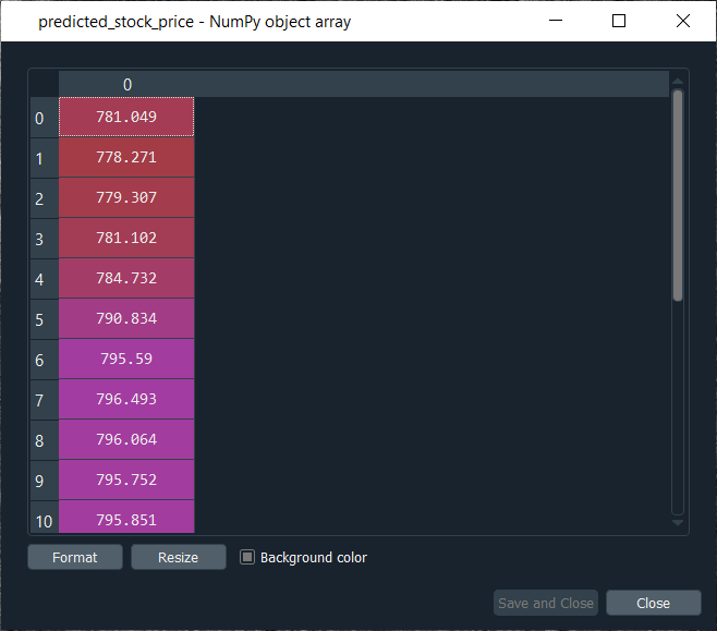
So, after executing the whole "Getting the predicted stock price of 2017" section, we will get the above output that contains the predictions, which is indeed in the range of Google Stock Prices in the month of January 2017. But we cannot realize it yet if it followed approximately the trend of the real Google Stock Price in January 2017. Next, we will move on to visualizing the results, which will actually witness the robustness of the model as we are going to see how our predictions follow the trends of the Google Stock Prices. Therefore, we will start by using the plt.plot function from the matplotlib.pyplot library and inside this plt.plot function, we will first need to input the name of the variable that contains the stored stock prices, which we want to plot, and these are contained in the real_stock_price variable. So, we first need to input the real_stock_price variable followed by adding our next argument, i.e., the color which we have chosen red for the real stock price, and then the last argument is the label for which we will plot some legends on the chart. Therefore we will use plt.legend function to display the legends. Here we have chosen 'Real Google Stock Price', so as to keep in mind that we are plotting not the whole real Google stock price between 2012 and the first month of 2017 instead we are plotting the real Google stock price in the first month of January 2017 because we only have the predictions of January 2017, so we just want to compare these two stock prices during this first month. Similarly, we will again use the plt.plot function to plot the predicted_stock_price variable that contains the stored predictions of the stock price for January 2017. It will be carried out in the same way as we did above, but will choose a different color, i.e., blue and label that is 'Predicted Google Stock Price'. Since we want to have a nice chart, so we will add a title to the chart for which we will use the plt.title function, and inside it, we will mention the title that we want to give to our chart, i.e. 'Google Stock Price Prediction'. Next, we will add the label to the x-axis as well as the y-axis, and to do that, we will use the plt.xlabel and plt.ylabel functions, each, respectively. Inside the plt.xlabel function, we will input the label that corresponds to the x-axis, i.e., 'Time' as we are plotting from 3rd January to 31st January and similarly inside the plt.ylabel, we will input the label that corresponds to the y-axis, i.e. 'Google Stock Price'. After this, we will add plt.legend function without any input so that we can include the legends in the chart followed by ending up with plt.show function to display the graph. Output: 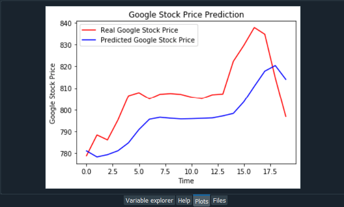
From the above input, we can see that we have the real Google stock price in red and our predicted Google stock price in blue. We also get a comparison of the real and the predicted Google stock prices for the whole month of January 2017. We have got the real Google stock price from the verified financial sources from the web. However, the predictions are coming from the RNN model that we just implemented. We can see in some parts our predictions are lagging behind the actual values. We can clearly see a big spike, like a stock time singularity, which is not followed by the predictions, and it is completely normal. Out model just lags behind because it cannot react to fast, nonlinear changes. The spike in the image is the stock time irregularity, is indeed a fast, nonlinear change to which our model cannot react properly, but that's totally fine because according to the Brownian Motion Mathematical Concept in financial engineering, the future variations of the stock price are independent of the past. And, therefore, the future variation that we see around the spike, well it is a variation that is indeed totally independent from the previous stock prices. But on the other hand, there is good news that out model reacts okay to smooth changes that happen on the Real Google Stock Price except for the spikes to which our model cannot react, but other than that, our Recurrent Neural Network reacts pretty well to these smooth changes. So, it can be concluded that in the parts of the predictions containing some spikes, well our predictions lag behind the actual values because our model cannot react to fast, nonlinear changes, whereas on the other hand, for the parts of the predictions containing smooth changes, well our model predicts pretty well as well as manages to follow the upward and downward trends. It manages to follow the upward trend, the stable trend, and again the upward trend on the Predicted Google Stock Price. Then there is a downward trend in the last financial days of January, and it started to capture it. So, we can say it make really good results that actually make pretty much sense in spite of spikes.
Next TopicKohonen Self-Organizing Maps
|
 For Videos Join Our Youtube Channel: Join Now
Feedback
- Send your Feedback to [email protected]
Help Others, Please Share


