Image Transforms in Image Recognition

Loading and transformation are two main concepts which are essential to do image recognition in PyTorch. Loading and transformation of the images is the starting step of the recognition process.

There are the following steps which are the step by step procedure to do loading and transformation:

Step 1:

In the first step, we install all the require library such as pip, torchvision, numpy, etc. If all the required library is already satisfied, then we import torch, and then we import datasets and transforms from torchvision. For plotting our dataset, we will import matplotlib.pyplot library and we will also import numpy to perform operations. The libraries are imported as:

Step 2:

In the second step, we load the MNIST dataset using the MNIST () method of datasets. In the first argument, we specified the root directory of our data as following

In the second argument, we set train='true'. We will do this to initialize the MNIST training dataset. After that, we set download ='true' and this will download a list into the data folder if it's not already there.

The last argument will be transform which is equal to transform1 argument that will initialize before the training_dataset. This argument dictates any image manipulation which you wish to apply on your images.

Note: Our MNIST images are 28*28 grayscale images which would imply that each image is a two dimensional number by array 28 pixels wide and 28 pixels long and each pixel intensity ranging from 0 to 255.

We must transform the image being in an array to a tensor. We will use Compose () method of transforms which will allow us to chain multiple transformations together . So our first transformation, which is passed as a first argument of composed, will transform.ToTensor(). This will convert our numpy array in the range of 0 to 255 to a float tensor in the range from 0 to 1.

We will also apply the normalize transformation with the help of normalize() method of transforms as:

In the normalize() method, we specified the mean which we are used to normalizing all channels of our tensor image, and we also specified the center deviation. Now, we call our training dataset as:

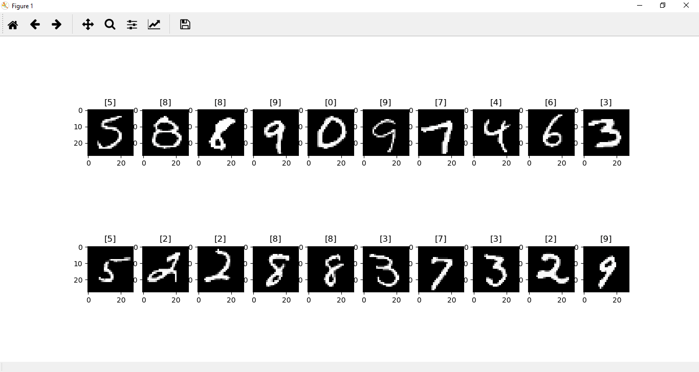
Step 3:

We will further analyze images within this dataset by plotting it. To plot the tensor image, we must change it back to numpy array. We will do this work in a function def im_convert() contain one parameter which will be our tensor image.

Before converting tensor to numpy array, first, we will clone it. It will create a new copy of tensor, and then we use the detach() function and then we will use numpy as:

Note: The tensor which will be converted into numpy array has a shape with the first, second, and third dimensions. The first dimension represents the color channel, and the second and the third dimensions represent the width and height of the image and pixels.

We know each image from the MNIST dataset is a grayscale corresponding to a single color channel with a width and height of 28*28 pixels. So, the shape would be (1, 28, 28).

Step 4:

For plotting our image, it is required that the image have a shape of (28, 28, 1). So, we will transpose our image by swapping axis zero, one, and two as:

This method swap axis 0 with axis 1 and axis 1 with axis 2.

Step 5:

In the next step, we de-normalized the image which we have to normalize before. Normalization is done by subtracting the mean and dividing by the standard deviation. We would multiply by the standard deviation and add the mean as:

To ensure that the range between 0 and 1, we used clip() function and pass zero and one as an argument. We will apply the clip function to a minimum value of 0 and the maximum value of 1 and return the image.

Step 6:

Now, we plot our MNIST dataset for better visualization. We will start by loading the image from training_loader(). The training loader is what we used to specify our training batches previously when training our neural network. For every epoch, we performed a single pass through the entire dataset. However, one epoch with sixty thousand training images would be too big to fit the computer all at once. So we will divide it into smaller batches using our train loader as:

The first argument is a dataset, which is equal to our training_dataset. The second argument is our batch size, which is equal to 100. The third argument, we set shuffle is equal to true.

Note: The batch size of 100 would take 600 iterations to complete one epoch and that each iteration it will update the weights of the neural network and minimizing the error.

Step 7:

In the next step, we wrap our train loader. It will create an object which allows us to go through the alterable training loader one element at a time. We access it one element at a time by calling next on our dataiter. The next () function will grab the first batch of our training data, and that training data will be split into images and labels as:

Step 8:

Now, we will plot the images in the batch along with their corresponding labels. This will be done with the help of figure function of plt and set fig size is equal to the tuple of integers 25*4, which will specify the width and height of the figure.

Now, we plot 20 MNIST images from our batch. We use add_subplot() method to add a subplot to the current figure and pass 2, 10, and idx as arguments of the function. Here two is no of rows, ten is no of columns, and idx is index.

Now, we will display our images with the help of im_show() function and give a title for each image plot as:

Finally call plt.show() and it will give us the expected result.

Complete code

Now, with the help of these label images, we will implement a neural network which will classify new test images.