| |

Linear RegressionLinear regression is used to predict the value of an outcome variable y on the basis of one or more input predictor variables x. In other words, linear regression is used to establish a linear relationship between the predictor and response variables. In linear regression, predictor and response variables are related through an equation in which the exponent of both these variables is 1. Mathematically, a linear relationship denotes a straight line, when plotted as a graph. There is the following general mathematical equation for linear regression: Here,
Steps for establishing the RegressionThe prediction of the weight of a person when his height is known, is a simple example of regression. To predict the weight, we need to have a relationship between the height and weight of a person. There are the following steps to create the relationship:
There is the following syntax of lm() function: Here,
Creating Relationship Model and Getting the CoefficientsLet's start performing the second and third steps, i.e., creating a relationship model and getting the coefficients. We will use the lm() function and pass the x and y input vectors and store the result in a variable named relationship_model. Example Output: Call: lm(formula = y ~ x) Coefficients: (Intercept) x 47.50833 0.07276 Getting Summary of Relationship ModelWe will use the summary() function to get a summary of the relationship model. Let's see an example to understand the use of the summary() function. Example Output:
Call:
lm(formula = y ~ x)

Residuals:
    Min      1Q  Median      3Q     Max
-38.948  -7.390   1.869  15.933  34.087

Coefficients:
            Estimate Std. Error t value Pr(>|t|)
(Intercept) 47.50833   55.18118   0.861    0.414
x            0.07276    0.39342   0.185    0.858

Residual standard error: 25.96 on 8 degrees of freedom
Multiple R-squared:  0.004257,	Adjusted R-squared:  -0.1202
F-statistic: 0.0342 on 1 and 8 DF,  p-value: 0.8579
The predict() FunctionNow, we will predict the weight of new persons with the help of the predict() function. There is the following syntax of predict function: Here,
Example Output: 1 59.14977 Plotting RegressionNow, we plot out prediction results with the help of the plot() function. This function takes parameter x and y as an input vector and many more arguments. Example Output: 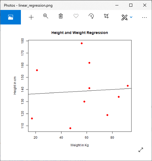
Next TopicR Multiple Linear Regression
|
 For Videos Join Our Youtube Channel: Join Now
Feedback
- Send your Feedback to [email protected]
Help Others, Please Share


