| |

R-Time Series AnalysisAny metric which is measured over regular time intervals creates a time series. Analysis of time series is commercially important due to industrial necessity and relevance, especially with respect to the forecasting (demand, supply, and sale, etc.). A series of data points in which each data point is associated with a timestamp is known as time series. The stock price at different points in a day in the stock market is the simplest example of the time series. The amount of rainfall in an area in different months of the year is another example of it. R provides several functions for creating, manipulating, and plotting time series data. In the R-object, the time series data is known as the time-series object. It is just like a vector or data frame. Creating a Time SeriesR provides ts() function for creating a Time Series. There is the following syntax of the ts() function: Here,
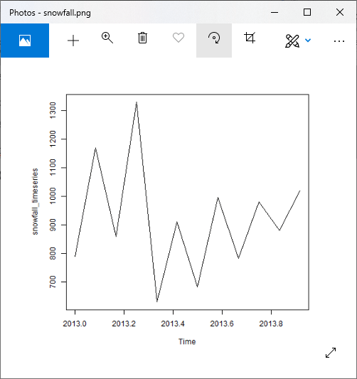
Let's see an example to understand how ts() function is used for creating Time Series. Example:In the below example, we will consider the annual snowfall details at a place starting from January 2013. We will create an R time series object for a period of 12 month and plot it. Output: 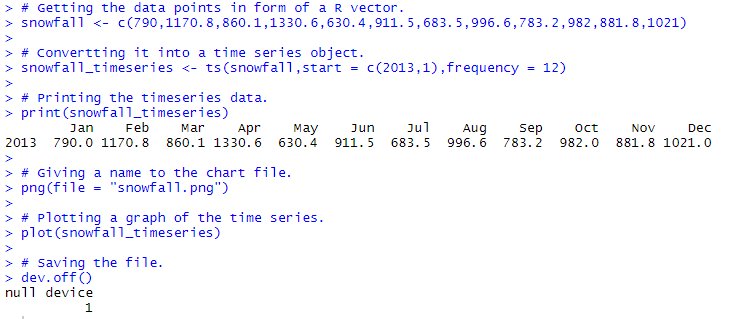
What is Stationary Time Series?A Stationary Time Series is a time series, if:
This means that it is devoid of or trendseasonal patterns, which resemble a random white noise regardless of the time interval observed. In simple words, a stationary time series is the one whose statistical properties like mean, variance, and autocorrelation, etc. are all constant over time. Extracting the trend, seasonality, and errorWe can decompose the time series by splitting it into three components, such as seasonality, trends, and random fluctuations. Time series decomposition is a mathematical process that transforms a time series into multiple time series. Seasonal: Patterns that repeat over a certain period of time Trend: An underlying trend of the matrices. Random: It is the residuals of the original time series after the seasonal and trend series are removed. Additive and Multiplicative DecompositionAdditive and Multiplicative decompositions are the models that are used for analyzing the series. When the seasonal variation seems to be constant means when the seasonal variation does not change at the time when the value of the time series increases, then we use the Additive model else we use the multiplicative model. 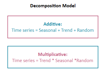
Let's see a step by step procedure to understand how we can decompose the time series using both Additive and Multiplicative model. For the additive model, we use ausbeer dataset, and for multiplicative, we use the AirPassengersdataset. Step 1: Load data and create time series For Additive Model Output: 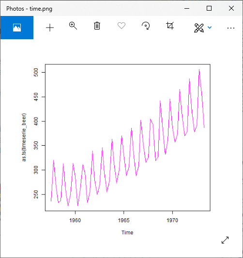
For Multiplicative Model Output: 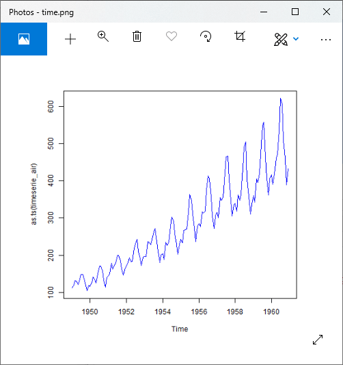
Step 2: Detecting the Trend For Additive Model Output1: 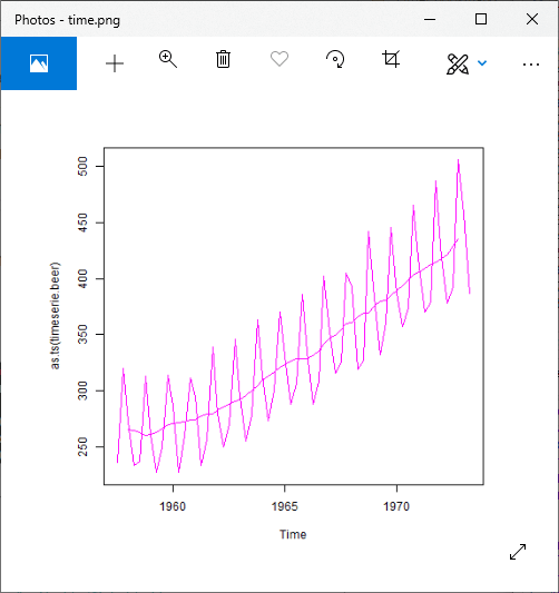
Output2: 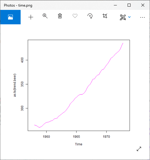
For Multiplicative Model: Output1: 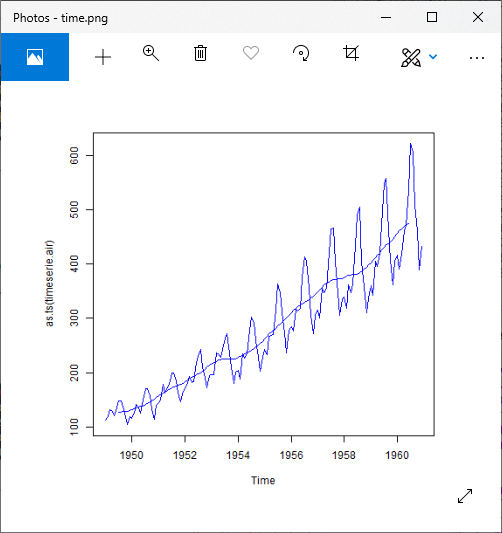
Output2: 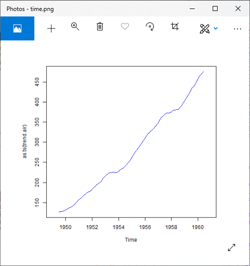
Step 3: Detrend of Time Series For Additive Model Output: 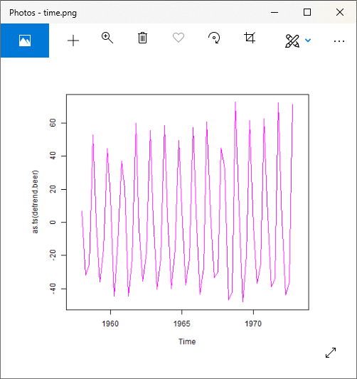
For Multiplicative Model Output: 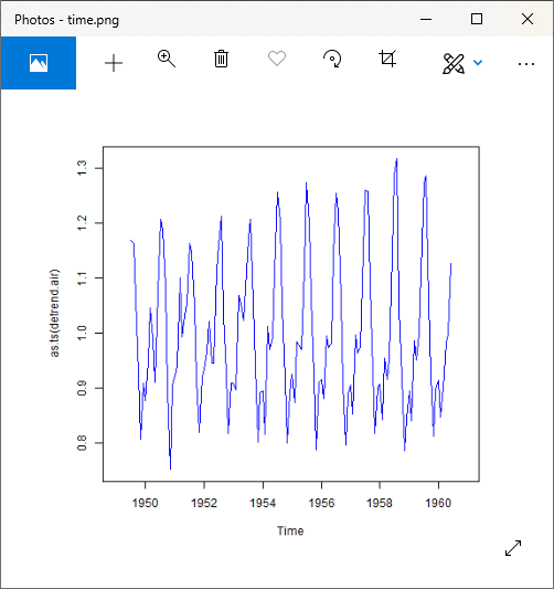
Step 4: Average the Seasonality For Additive Model Output: 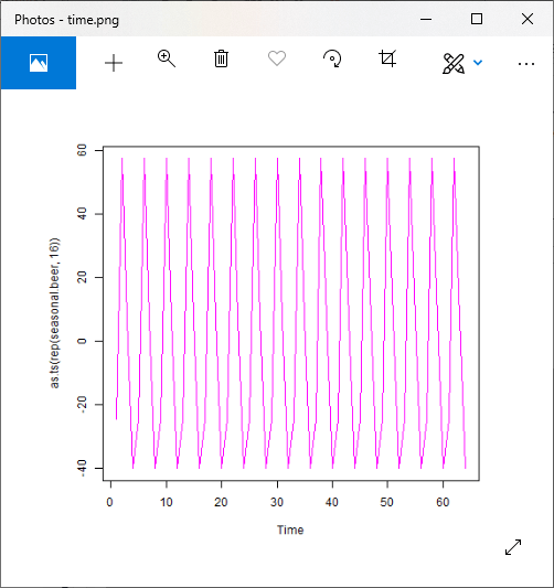
For Multiplicative Model Output: 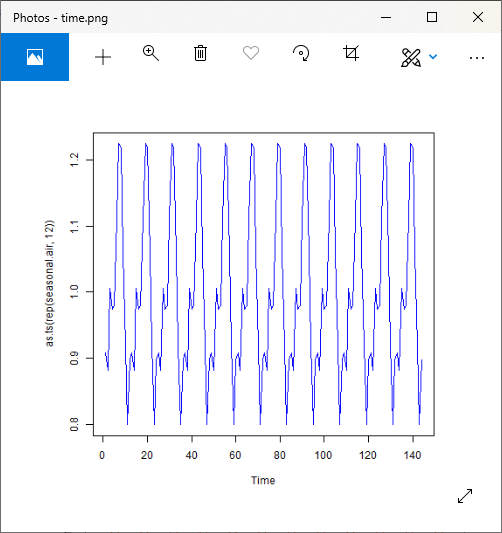
Step 5: Examining the Remaining Random Noise For Additive Model Output: 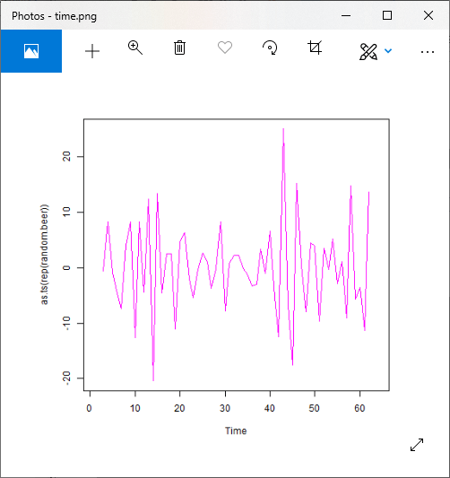
For Multiplicative Model Output: 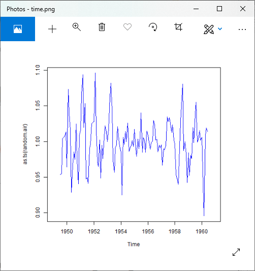
Step 5: Reconstruction of Original Signal For Additive Model Output1: 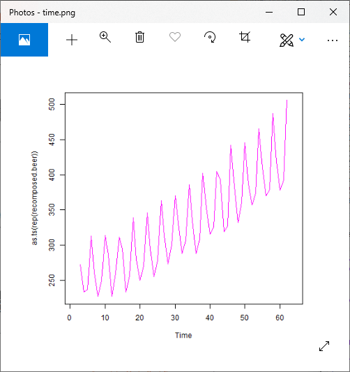
For Multiplicative Model Output: 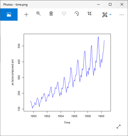
Time Series Decomposition using decompose()For Additive Model Output: 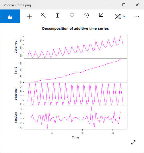
For Multiplicative Model Output: 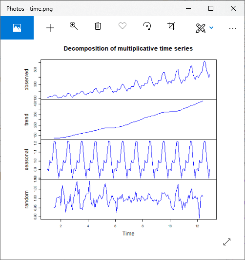
Next TopicR-Random Forest
|
 For Videos Join Our Youtube Channel: Join Now
Feedback
- Send your Feedback to [email protected]
Help Others, Please Share


