| |

Extended Function Point (EFP) MetricsFP metric has been further extended to compute:
Feature Points
Feature Point Calculations
The feature point is thus calculated with the following formula: FP = Count-total * [0.65 + 0.01 *∑(fi)] where count-total is obtained from the above table. CAF = [0.65 + 0.01 * ∑(fi)] and ∑(fi) is the sum of all 14 questionnaires and show the complexity adjustment value/factor-CAF (where i ranges from 1 to 14). Usually, a student is provided with the value of ∑(fi) . 6. Function point and feature point both represent systems functionality only. 7. For real-time applications that are very complex, the feature point is between 20 and 35% higher than the count determined using function point above. 3D function pointsThree dimensions may be used to represent 3D function points?data dimension, functional dimension, and control dimension. 2. The data dimension is evaluated as FPs are calculated. Herein, counts are made for inputs, outputs, inquiries, external interfaces, and files. 3. The functional dimension adds another feature-Transformation, that is, the sequence of steps which transforms input to output. 4. The control dimension that adds another feature-Transition that is defined as the total number of transitions between states. A state represents some externally observable mode 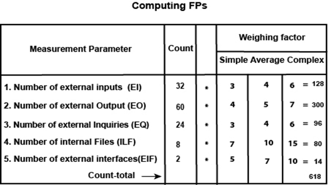
Now fi for average case = 3. So sum of all fi (i ←1 to 14) = 14 * 3 = 42 and feature point = (32 *4 + 60 * 5 + 24 * 4 + 80 +14) * 1.07 + {12 * 15 *1.07} Example: Compute the 3D-function point value for an embedded system with the following characteristics:
Assume complexity of the above counts is high. Solution: We draw the Table first. For embedded systems, the weighting factor is complex and complexity is high. So, 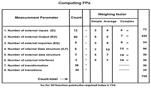
Next TopicData Structure Metrics
|
 For Videos Join Our Youtube Channel: Join Now
Feedback
- Send your Feedback to [email protected]
Help Others, Please Share


