Jelinski and Moranda Model

The Jelinski-Moranda (JM) model, which is also a Markov process model, has strongly affected many later models which are in fact modifications of this simple model.

Characteristics of JM Model

Following are the characteristics of JM-Model:

1. It is a Binomial type model
2. It is certainly the earliest and certainly one of the most well-known black-box models.
3. J-M model always yields an over-optimistic reliability prediction.
4. JM Model follows a prefect debugging step, i.e., the detected fault is removed with certainty simple model.
5. The constant software failure rate of the J?M model at the i^th failure interval is given by:

        λ(t_i) = ϕ [N-(i-1)],     i=1, 2... N .........equation 1

Where

ϕ=a constant of proportionality indicating the failure rate provided by each fault

N=the initial number of errors in the software

t_i=the time between (i-1)^th and (i)^th failure.

The mean value and the failure intensity methods for this model which belongs to the binominal type can be obtained by multiplying the inherent number of faults by the cumulative failure and probability density functions (pdf) respectively:

            μ(t_i )=N(1-e^-ϕt_i)..............equation 2

And

            €(t_i)=Nϕe^-ϕt_i.............equation 3

Those characteristics plus four other characteristics of the J-M model are summarized in table:

Measures of Reliability name	Measures of Reliability formula
Probability density function	f(ti)= ϕ[N-(i-1]e-ϕ[N-(i-1)]ti
Software Reliability function	R(ti)= e-ϕ[N-(i-1)]ti
Failure rate function	λ(ti)= ϕ[N-(i-1)]
Mean time to failure function
Mean value function	µ(ti )=N(1-e-ϕti)
Failure Intensity function	€(ti )=Nϕe-ϕti
Median	m={ϕ[N-(i-1)]} -1 In2
Cumulative Distribution function	f(ti)=1-e-ϕ[N-(i-1)]ti

Assumptions

The assumptions made in the J-M model contains the following:

1. The number of initial software errors is unknown but fixed and constant.
2. Each error in the software is independent and equally likely to cause a failure during a test.
3. Time intervals between occurrences of failure are separate, exponentially distributed random variables.
4. The software failure rate remains fixed over the ranges among fault occurrences.
5. The failure rate is corresponding to the number of faults that remain in the software.
6. A detected error is removed immediately, and no new mistakes are introduced during the removal of the detected defect.
7. Whenever a failure appears, the corresponding fault is reduced with certainty.

Variations in JM Model

JM model was the first prominent software reliability model. Several researchers showed interest and modify this model, using different parameters such as failure rate, perfect debugging, imperfect debugging, number of failures, etc. now, we will discuss different existing variations of this model.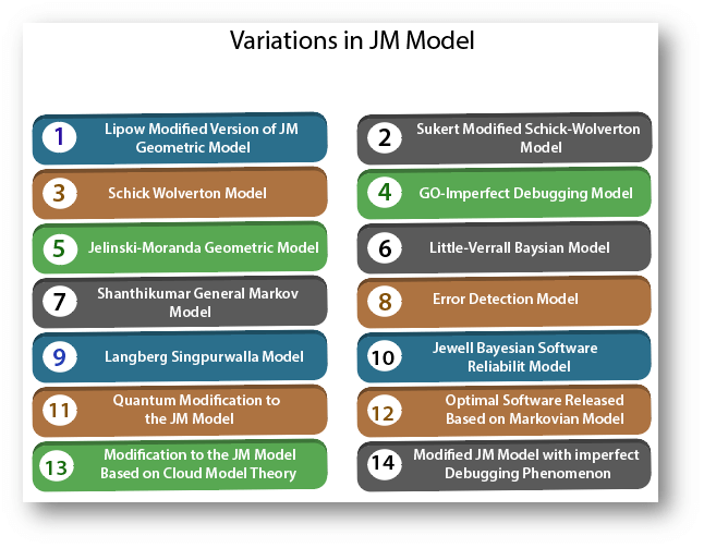

1. Lipow Modified Version of Jelinski-Moranda Geometric Model

It allows multiple bugs removal in a time interval. The program failure rate becomes

            λ(t_i)=DK^n_i-1

Where n_i-1 is the cumulative number of errors found up to the (i-1)st time interval.

2. Sukert Modified Schick-Wolverton Model

Sukert modifies the S-W model to allow more than one failure at each time interval. The program failure rate becomes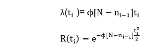

Where n_i-1 is the cumulative number of failures at the (i-1)th failure interval.

3. Schick Wolverton Model

The Schick and Wolverton (S-W) model are similar to the J-M model, except it further consider that the failure rate at the ith time interval increases with time since the last debugging.

Assumptions

• Errors occur by accident.
• The bug detection rate in the defined time intervals is constant.
• Errors are independent of each other.
• No new bugs are developed.
• Bugs are corrected after they have been detected.

In the model, the program failure rate method is:

            λ (t_i)= ϕ[N-(i-1)] t_i

Where ϕ is a proportional constant, N is the initial number of bugs in the program, and t_i is the test time since the (i-1)st failure.

4. GO-Imperfect Debugging Model

Goel and Okumoto expand the J-M model by assuming that an error is removed with probability p whenever a failure appears. The program failure rate at the ith failure interval is

            λ (t_i)= ϕ[N-p(i-1)]
            R(t_i)=e^{-ϕ[N-p(i-1)]-t_i)}

5. Jelinski-Moranda Geometric Model

This model considers that the program failure rate function is initially a constant D and reduce geometrically at failure time. The program failure rate and reliability method of time between failures at the ith failure interval are

            λ (t_i)=DK^i-1
            R(t_i)=e^-DKi-1_ti)

Where k is Parameter of geometric function, 0<k<1

6. Little-Verrall Bayesian Model

This model considers that times between failures are independent exponential random variables with a parameter € i=1, 2 ....n which itself has parameters Ψ(i) and α reflecting programmer quality and function difficulty having a prior gamma distribution.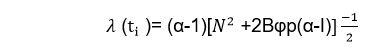

Where B represents the fault reduction factor

7. Shanthikumar General Markov Model

This model considers that the failure intensity functions as the number of failures removed are as the given below

            λ _SG(n, t) = Ψ(t) (N₀-n)

Where Ψ (t) is proportionality constant.

8. An Error Detection Model for Application during Software Development

The primary feature of this new model is that the variable (growing) size of a developing program is accommodated so that the quality of a program can be predicted by analyzing a basic segment.

Assumptions

This model has the following assumptions along with the JM model assumptions:

1. Any tested initial portion of the program describes the entire program for the number and nature of its incipient errors.
2. The detect-ability of a mistake is unaffected by the "'dilution" incurred when the initially tested method is augmented by new code.
3. The number of lines of code which exists at any time is known.
4. The growth function and the bug detection process are independent.

9. The Langberg Singpurwalla Model

This model shows how several models used to define the reliability of computer software can be comprehensively viewed by adopting a Bayesian point of view.

This model provides a different motivation for a commonly used model using notions from shock models.

10. Jewell Bayesian Software Reliability Model

Jewell extended a result by Langberg and Singpurwalla (1985) and made an expansion of the Jelinski-Moranda model.

Assumptions

1. The testing protocol is authorized to run for a fixed length of time-possibly, but not certainly, coinciding with a failure epoch.
2. The distribution of the unknown number of shortage is generalized from the one-parameter Poisson distribution by considering that the parameter is itself a random quantity with a Beta prior distribution.
3. Although the estimation of the posterior distributions of the parameters leads to complex expressions, we show that the calculation of the predictive distribution for undetected bugs is straightforward.
4. Although it is now identified that the MLE's for reliability, growth can be volatile, we show that, if a point estimator is needed, the predictive model is easily calculated without obtaining the full distribution first.

11. Quantum Modification to the JM Model

This model replaces the JM Model assumption, each error has the same contribution to the unreliability of software, with the new assumption that different types of errors may have different effects on the failure rate of the software.

Failure Rate: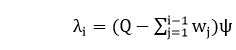

Where

Q = initial number of failure quantum units inherent in a software

Ψ = the failure rate corresponding to a single failure quantum unit

w_j= the number of failure-quantum units of the ith fault, i.e., the size of the ith failure-quantum

12. Optimal Software Released Based on Markovian Software Reliability Model

In this model, a software fault detection method is explained by a Markovian Birth process with absorption. This paper amended the optimal software release policies by taking account of a waste of a software testing time.

13. A Modification to the Jelinski-Moranda Software Reliability Growth Model Based on Cloud Model Theory

A new unknown parameter θ is contained in the JM model parameters estimation such that θɛ [θ_L, θ_∪]. The confidence level is the probability value (1-α) related to a confidence interval. In general, if the confidence interval for a software reliability index θ is achieved, we can estimate the mathematical characteristics of virtual cloud C(Ex, En, He), which can be switched to system qualitative evaluation by X condition cloud generator.

14. Modified JM Model with imperfect Debugging Phenomenon

The modified JM Model extends the J-M model by relaxing the assumptions of complete debugging process and types of incomplete removal:

1. The fault is not deleted successfully while no new faults are introduced
2. The fault is not deleted successfully while new faults are created due to incorrect diagnoses.

Assumptions

The assumptions made in the Modified J-M model contain the following:

• The number of initial software errors is unknown but fixed and constant.
• Each error in the software is independent and equally feasible to cause a failure during a test.
• Time intervals between occurrences of failure are independent, exponentially distributed random variables.
• The software failure rate remains fixed over the intervals between fault occurrences.
• The failure rate is proportional to the number of errors that remain in the software.
• Whenever a failure occurs, the detected error is removed with probability p, the detected fault is not entirely removed with probability q, and the new fault is generated with probability r. So it is evident that p+q+r=1and q≥r.

List of various characteristics underlying the Modified JM Model with imperfect Debugging Phenomenon