Survival Analysis Using Machine Learning

Survival analysis is a statistical method used to analyze time-to-event data. It involves the study of the time it takes for an event of interest to occur, such as the time until a patient experiences a disease progression or death. Machine learning can be used in survival analysis to model the relationship between the event of interest and the predictor variables.

One popular approach to survival analysis using machine learning is the Cox proportional hazards model. This model allows for the estimation of the hazard function, which represents the instantaneous probability of the event of interest occurring at any given time, based on the predictor variables. The Cox proportional hazards model assumes that the hazard function is proportional across different levels of the predictor variables.

Another approach to survival analysis using machine learning is the random survival forest (RSF) model. The RSF model is an extension of the random forest algorithm that is specifically designed for survival analysis. The RSF model uses decision trees to split the data into subgroups based on the predictor variables and estimates the survival probability for each subgroup.

There are also deep learning-based approaches to survival analysis, such as the DeepSurv model, which uses a neural network to estimate the hazard function. DeepSurv is designed to handle large datasets with high-dimensional predictor variables and can capture complex relationships between the predictors and the event of interest.

Machine learning-based survival analysis can be used in a variety of applications, such as predicting patient outcomes, estimating the time until equipment failure, or modelling the survival of a species in an ecosystem. It is important to note that these models require careful validation and interpretation, as survival analysis can be influenced by censored data and other biases.

For the sake of better understanding, we will try to analyze the Breast Cancer (METABRIC) dataset.

Code Implementation

• Importing Libraries:

• Time to Event Data

Every topic has a time period and an event in the time-to-event data. The amount of time till the occurrence is measured. This time frame might be the span between a patient's cancer diagnosis or the beginning of therapy and their death, or it could be the span between a tumour's spread or local recurrence. It's not necessary for the incident to be unfavourable. Recovery or anything else uplifting can be included. Time-to-event data are sometimes referred to be survival or failure time data as a result of the instances of time-to-event data that were initially researched. The statistical methods created to address these are referred to as survival analysis.

The analysis in this article makes use of the Breast Cancer (METABRIC) dataset. It includes the clinical characteristics of 2,509 breast cancer patients as well as information on the intervals between diagnoses and recurrence and death.

• Loading the Dataset

Output:

• EDA

The METABRIC dataset contains 2,509 distinct breast cancer patients, as was previously noted. These patients' mean age at diagnosis, which ranges from 21.9 to 96.3, is 60.4. Patients received either a mastectomy, which involves removing all breast tissue from a breast or breast-conserving surgery (removal of a part of the breast that has cancer). Although breast sarcomas are an extremely rare kind of breast cancer that accounts for less than 1% of all breast cancers, there are 2,506 breast cancer patients and three breast sarcoma patients in the dataset. Invasive ductal carcinoma (IDC), which accounts for 1865 cases of breast cancer, is the most prevalent histological subtype. IDC accounts for 80% of all breast cancer diagnoses, making it the most prevalent kind. These indications demonstrate how effectively this dataset captures real-world circumstances.

Output: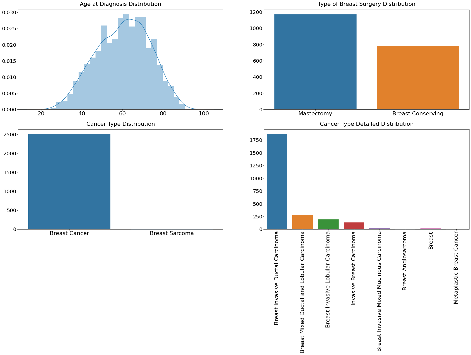

In the dataset, there are two events reported. The outcomes are relapse and overall survival status (Relapse Free Status). Moreover, those events have two durations: overall survival (months) and relapse-free status (Months). These two occurrences and their durations form the basis of the survival analysis. Although the distributions of the two durations are extremely similar, the distribution of events is slightly different. In a survival event, the label "Deceased" is more frequent, indicating that the event occurred, whereas the label "Not Recurred" indicates that the event did not occur in a relapse event.

Output: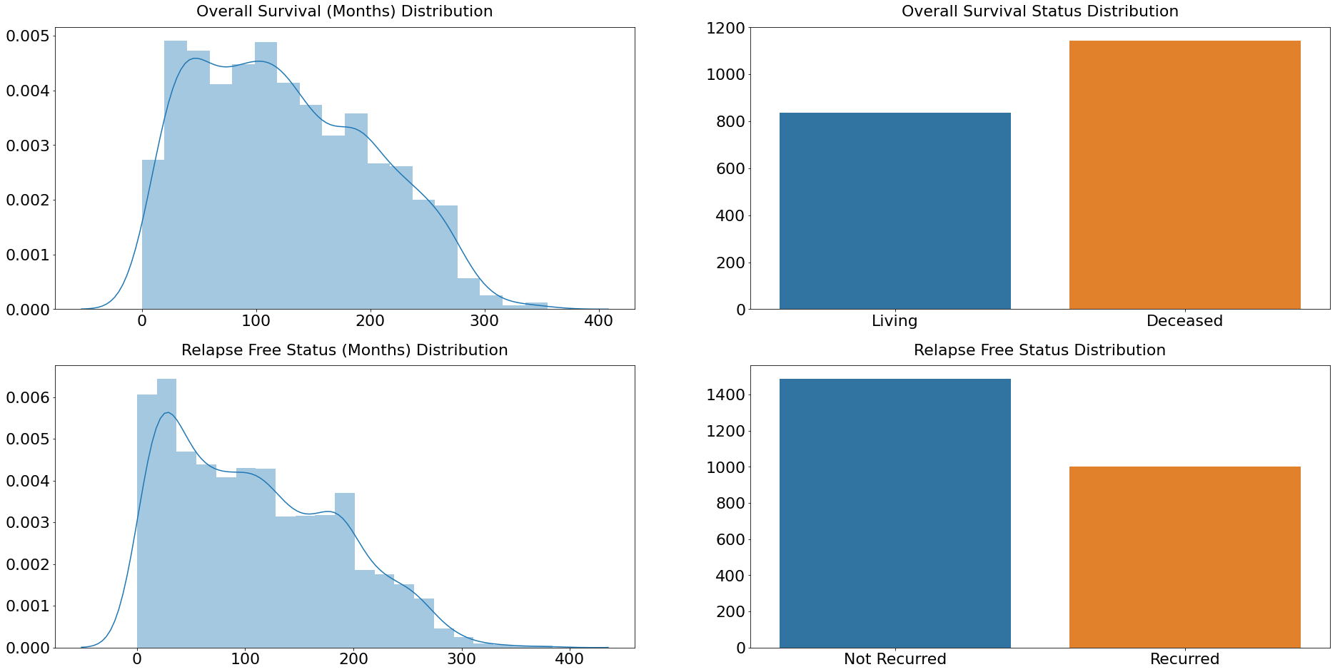

Clinical profiles of the patients are additional characteristics in the dataset. These characteristics include the tumour's cellularity, whether the patient has received chemotherapy, hormone treatment, radiotherapy, or not, the patient's ER, PR, and HER2 status, as well as the tumour's size, stage, and histologic subtype. These characteristics can be included as variables in models of survival analysis, although doing so necessitates additional preprocessing and cleaning.

Output: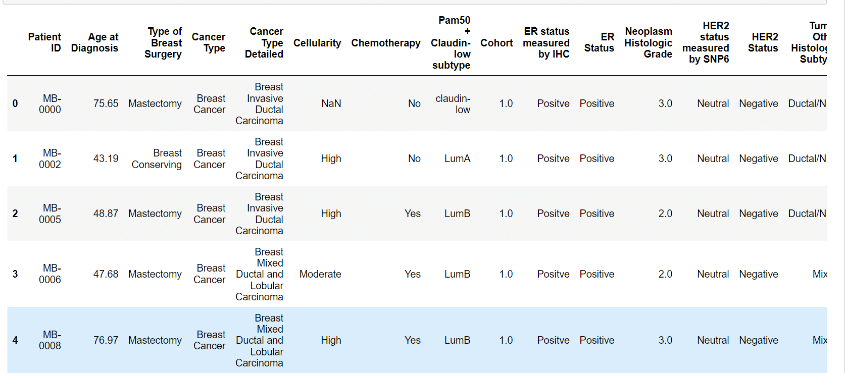

• Preprocessing and Cleaning

Just five columns are free of missing values, while 29 columns have missing values. Sex, Cancer Type Details, Cancer Type, Oncotree Code, and Patient ID are those columns. Others don't provide any information; however, Cancer Type and Cancer Type Detailed can be quite helpful for imputation.

Output: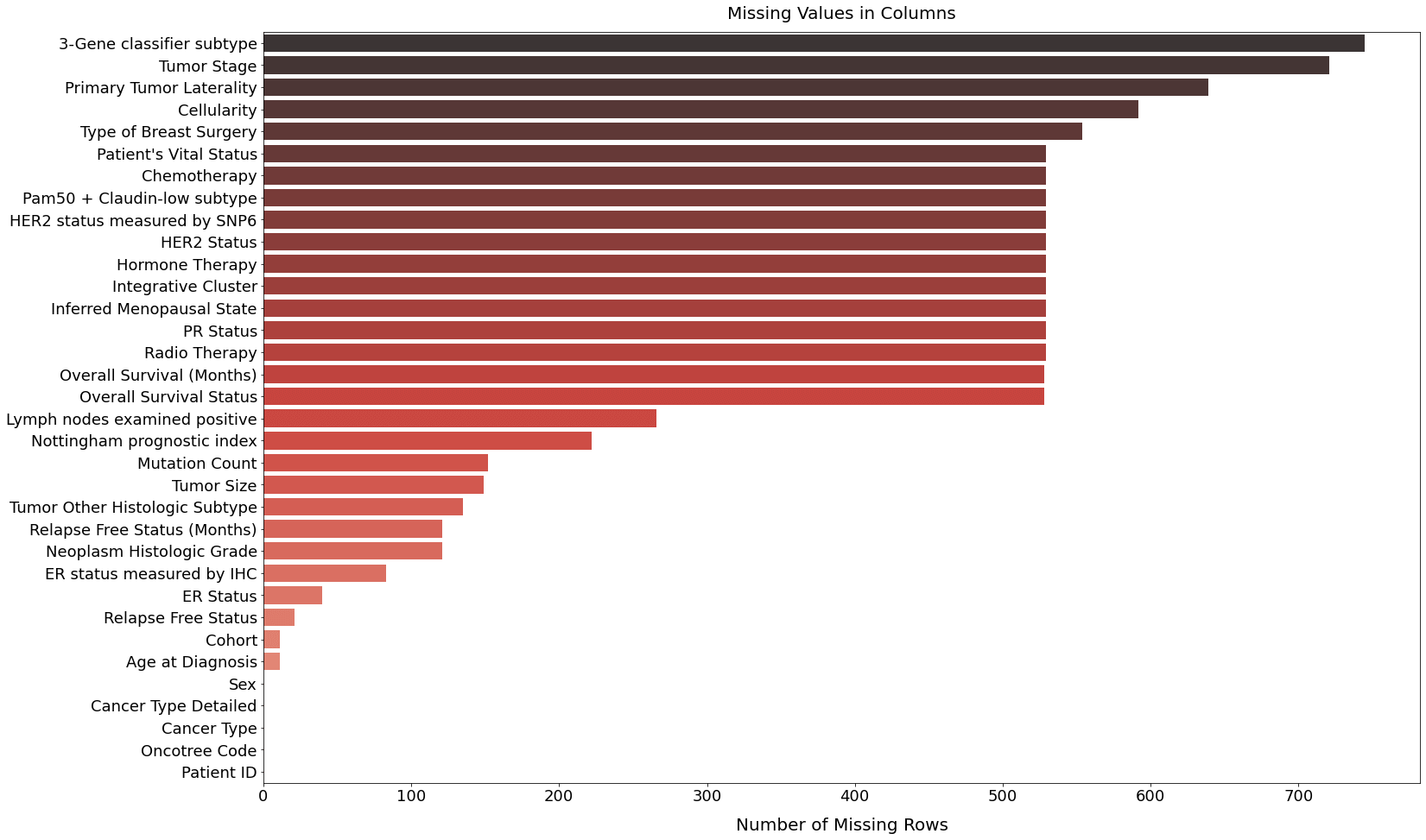

At the imputation stage, dependencies between distinct columns are taken advantage of. Missing values in duration columns are filled with the most frequent values of Cancer Type Detailed Event groups, whereas missing values in event columns are filled with their most frequent value. The most frequent values of their measurement technique columns are used to fill in the gaps in the ER, PR, and HER2 Status columns (ER status is measured by IHC and HER2 status is measured by SNP6). The most prevalent values in the Cancer Type Detailed categories are used to fill in the missing values for Chemotherapy, Hormone treatment, and Radiotherapy. Based on their interdependence, the modes or medians of various groups are used to fill in the missing values in other columns. The iterative filling is used for some columns that couldn't be completed in one go. Last but not least, the Patient's Vital Status field is removed because it provides no more data for the study.

Object type columns are label encoded and converted to uint8 at the end of the preprocessing procedure to save memory. Because LabelEncoder can label "event happened" as 0, two event columns?Overall Survival Status and Relapse Free Status-are manually encoded. This completes the notebook's introductory section and prepares the data for the models.

Now that each column is a number, their correlations may be determined. Because several attributes depend on one another, there are some significant correlations above 0.6 and below -0.6. One of these should be deleted since Cellularity and Integrative Cluster have one perfect positive association. One critical factor to take into account is the dependency of the overall survival status on the relapse-free status. For this reason, such traits shouldn't be employed as covariates. The Sex column corresponds to an empty row and column at the end. Given that all of the patients are women, the Sex column has no variance and no associations. Hence, they are both empty.

Output: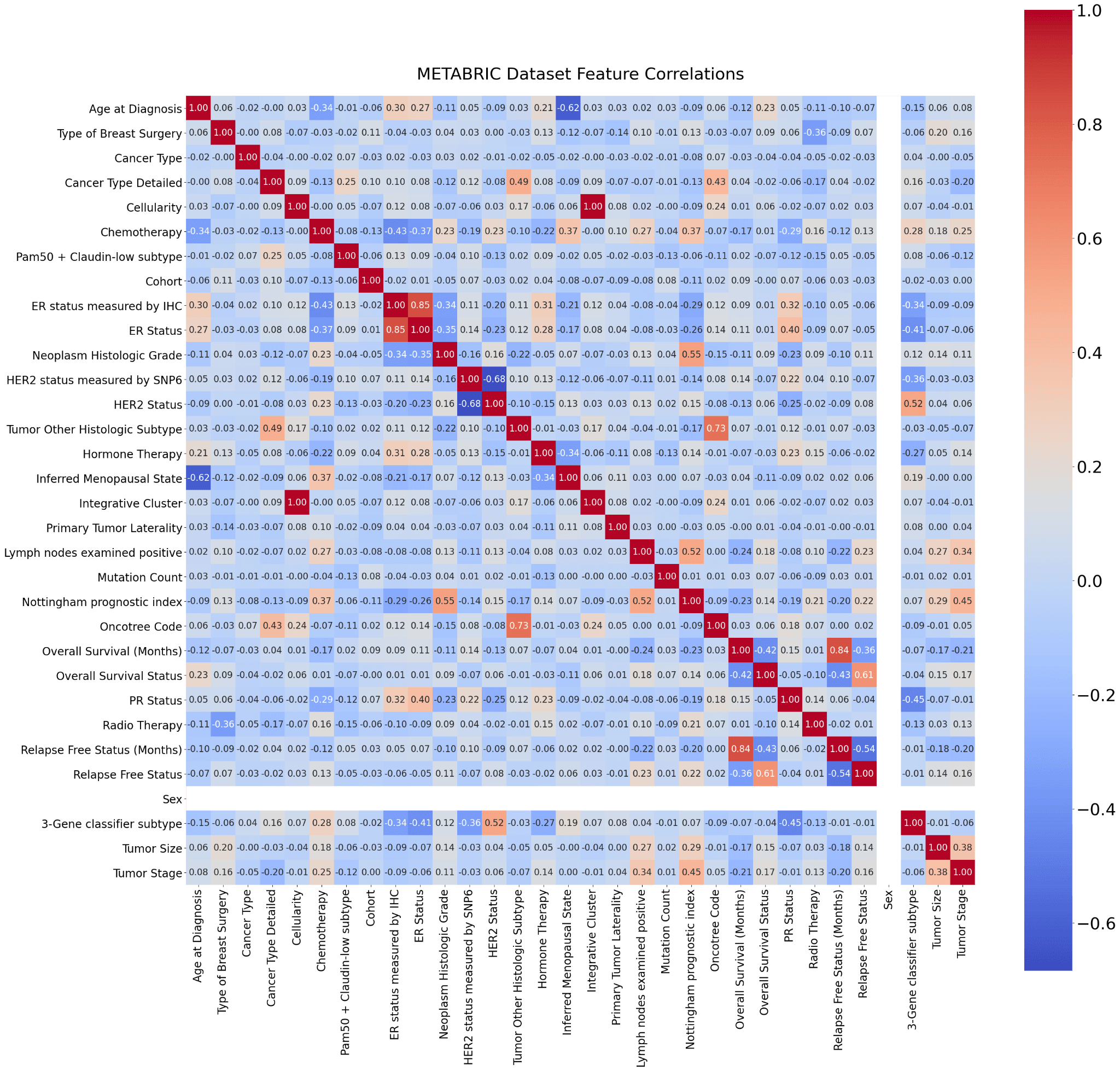

Theory

Survival Function

The aim of the group of techniques associated with survival analysis is to calculate the survival function using survival data. Let T represent a (potentially unlimited, but always positive) random time drawn from the research dataset. S(t), or the survival function of a population, is given by the formula S(t)=Pr(T>t). The likelihood that the event hasn't happened yet at time t, or more accurately, the probability of living past time t, is defined simply by the survival function.

The random lifespan, T, which cannot be negative, is taken from the dataset under investigation. The survival function S(t), which is a non-increasing function of t, produces values between 0 and 1. At the beginning of the time period (t=0), no subject has yet encountered the event. The chance S(0) of living past time zero is thus 1. As everyone would eventually encounter the event of interest if the research period were infinite, S(∞)=0 since the chance of surviving would eventually reach zero. Although, in principle, the survival function is smooth, in reality, events are observed over a certain time period, such as days, weeks, months, etc., making the survival function's graph resemble a step function.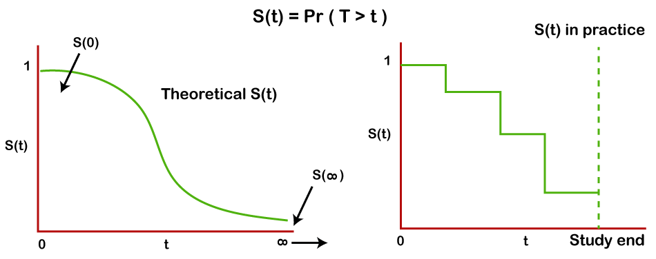

Hazard Function

The likelihood of the event occurring at time t is provided by the hazard function h(t), given that the event has not yet happened. The probable instantaneous occurrence of the event per unit of time is described. It is said as follows:

𝑃𝑟(𝑡≤𝑇≤𝑡+𝛿𝑡|𝑇>𝑡)

This amount is divided by the interval t since it becomes zero as t becomes smaller. The hazard function at time t, h(t), is defined as follows: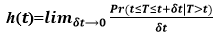

As a result, hazard function models show which time periods have the greatest or smallest likelihood of an incident. The danger function does not have to start at 1 and decrease to 0 like the survival function does. Typically, the danger rate fluctuates over time. It might begin anywhere and fluctuate over time.

Censoring

Understanding filtering is a fundamental element in survival analysis. There are two sorts of observations in survival analysis:

• Event occurred, and it could be measured at the time it did.
• The event wasn't seen throughout that time, and only the total number of days that it wasn't observed is known (censored)

There are two groups, one in which the time till the occurrence is precisely known and the other in which it is not. The event of interest did not occur for a specific period of time in the case of the second group. These people are the subjects of censorship. Making the decision to disregard the filtered group is a typical error. Although it is unknown if the event would have happened had we watched the person for a longer period of time, the fact that it didn't indicates that the event was not likely to happen to that person.

We can't follow someone around indefinitely, which is one reason for censorship. The research must come to an end at some time, and not everyone will have witnessed the occurrence. Another frequent factor is the loss of research participants for follow-up. We refer to this as random censoring. When follow-up is discontinued due to circumstances outside the investigator's control, it happens.

In a survival analysis, censored observations add to the total number of people at risk up until the point at which they were no longer being tracked. One benefit of this approach is that it is not necessary for everyone to be watched for the same amount of time. The analysis can account for the possibility that the follow-up times for each observation vary.

Right, left, and interval censoring is the three different forms of censorship.

Right Censoring

The most typical kind of censorship is right censoring. That happens when the survival time at the proper side of the follow-up period is incomplete. Take the situation where three patients (A, B, and C) are engaged in a clinical trial that lasts for a while (study end - study start). The graphic below shows the distinct paths of 3 patients.

• Patient A: Has an incident before the research is through.
• Patient B: Lives to see the study's conclusion.
• Patient C: Leaves the experiment.

Patient A doesn't need to be censored since we know exactly how long they have to live or how long they have till they die. But, because we don't know the patient's precise survival duration, Patient B needs to be censored. Just their survival during the research is known. As Patient C left the trial before it was finished, they, too, need to be censored. Since we don't know the patient's actual survival duration, we can only assume that they lived up until the point of withdrawal. The real survival times in right censoring will always be equal to or longer than the observed survival times.

Output: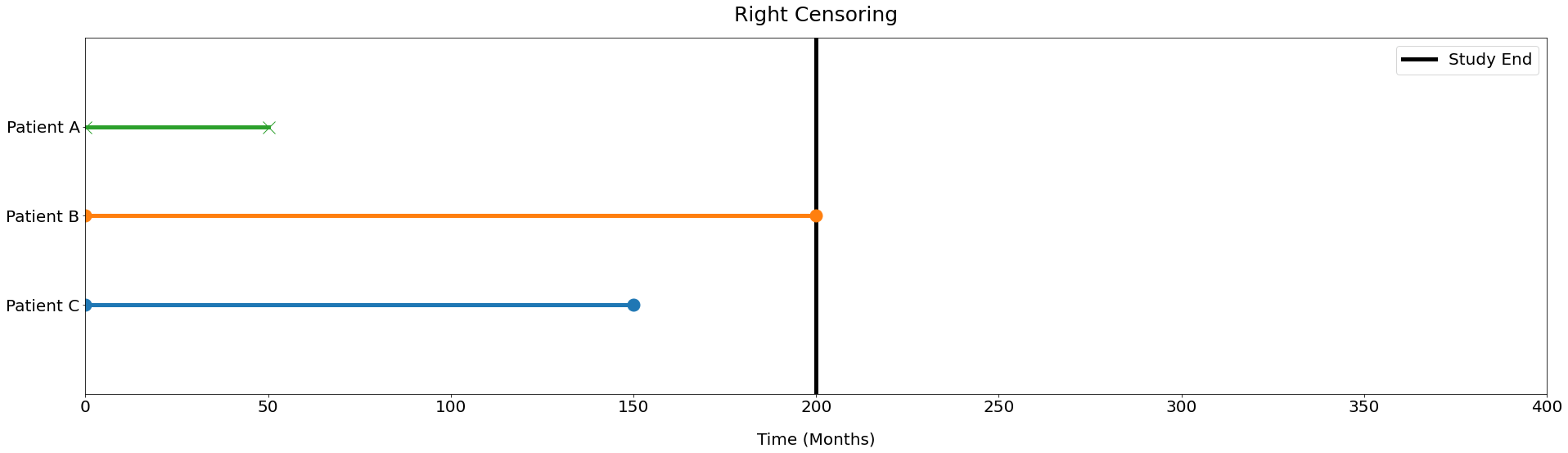

Left Censoring

When we are unable to determine the exact moment an incident took place, left-censoring happens. The data cannot be left censored if the event is death for obvious reasons. Virus testing is a prime illustration. For instance, if we have been monitoring a person and have noted a positive viral test, but we are unsure about the precise moment the person was exposed to the disease. Just the fact that there was some exposure between zero and the testing period is known.

Interval Censoring

If, like in the case of the virus test, we had tested the person at a time point (t1) and the results were negative, the scenario would be as follows. However, at a later time point (t2), the person's test result was positive. In this instance, we are aware that the person was exposed to the virus between t1 and t2, but we are unsure of the precise moment of the exposure. This can serve as a good interval censoring example.

Evaluation

An elegant solution to the filtering of the data as well as the frequently skewed distributions of survival times, is to formulate survival analysis as a ranking issue. Not only can the survival times of two subjects be sorted if they are both uncensored, but also if one of them has a shorter uncensored duration than the other.

The concordance index (CI), often known as the c-index, is one of the most frequently used performance indicators of survival models for the reasons stated above. It may be understood as the proportion of all subject pairings among all subjects whose estimated survival times are appropriately arranged. In other words, it is the likelihood that the expected and observed survival rates would agree. One way to spell it is as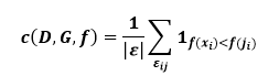

use the indicator function 1ab=1 if ab, and 0 otherwise. The model f's expected survival time for a subject I is expressed as f(xi). The fact that this index may be used with continuous output variables and take into account data censoring makes it a generalization of the Wilcoxon-Mann-Whitney statistics and, consequently, of the area under the ROC curve (AUC) to regression issues. C = 1 denotes perfect prediction accuracy, whereas C = 0.5 is equivalent to a random predictor, much like the AUC.

The concordance index is implemented in the Lifelines package. It requires 3 parameters: projected scores (array-like partial hard rates or survival times), event times (object with durations similar to an array), and event seen (array-like binary event data). Using the signature lifelines.utils.concordance index(event times, predicted scores, event observed), the scoring function may be invoked. Return value is the average of how frequently a model asserts that X is larger than Y when in fact, X is greater than Y in the observed data. The suppressed values are likewise handled by this function.

Ranking event probability at certain times is another method of assessing a survival model. The function time-dependent roc auc score, which is described below, can be used for this procedure. It first transforms ground truth labels with a shape of (n samples, 1) into a matrix with a shape of (n samples, n evaluation times). Following that, sklearn.metrics.roc auc score is determined each time (column).

Survival Models

A certain dataset format is needed for survival analysis models:

• E is the event indicator such that Ei=0 in the case of censorship and Ei=1 if an event occurs.
• T is the measured time.
• An n-dimensional feature vector is X. (covariates)

The three primary categories of conventional methods for estimating survival are non-parametric, semi-parametric, and parametric techniques. The premise behind parametric approaches is that the distribution of survival times fits into particular probability distributions. These techniques include Weibull, exponential, and lognormal distributions, among others. These models often employ specific maximum likelihood estimations to predict the parameters. There are no dependencies on the shape of the parameters in the underlying distributions when using non-parametric approaches. The non-parametric technique is typically used to present an average picture of the population of individuals and to describe survival probability as a function of time. The Kaplan-Meier estimator is the most often used univariate approach. The Cox regression model, which is based on both parametric and non-parametric components, relates to semi-parametric approaches.

Cross-validation is performed using a StratifiedKFold with five splits. Cancer Type Detailed is stratified. However, because of the rarity of specific values, some values are not properly stratified. A holdout test set using the same split approach is employed for the final assessment.

Kaplan-Meier Estimate (Non-parametric Model)

The Kaplan-Meier estimate is the most used non-parametric method for estimating the survival function. Non-negative regression and density estimation for a single random variable (initial event time) in the presence of censoring is another approach to thinking about survival analysis. In the case of censoring, Kaplan-Meier is a non-parametric density estimate (empirical survival function). This model has the benefit of being extremely adaptable, and model complexity increases with the number of observations. There are two drawbacks, though:

1. It is difficult to define how individual differences in survival functions are dependent on the profiles since it is difficult to add variables. The primary method is to fit several models to various subpopulations and compare them. This is challenging to scale, though, as the number of attributes and the values of those characteristics increase.
2. The mechanisms of survival are not efficient. They are piecewise constant, in particular. As the sample size increases, they become closer to a smooth estimator, but for small samples, they are still far from it. The idea that the death probability may suddenly increase or decrease is not entirely believable. Moreover, it will assign a survival probability of 1 to the range [0,t] if there are no death observations during that time, which may not be what you want. There are techniques for kernel smoothing, which may be used to improve the survival function. However, it can be difficult to understand the results.

The Kaplan-Meier estimator's main principle is to divide the estimation of the survival function S(t) into more manageable stages based on the observed event timings. Using the following formula, the chance of living until the end of each period is calculated: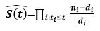

Kaplan-Meier Fitter is first fitted to the whole dataset, despite the fact that data is divided into the train, validation, and test sets. This is one way to utilize the Kaplan-Meier estimate to acquire a broad overview of the population. For both Overall Survival Status and Relapse Free Status events, the estimated S(t) is displayed as a stepwise function of the total population of people.

The likelihood that a patient will still be alive or will not have relapsed after t months is shown on the y-axis, with t months being represented on the x-axis. To describe how uncertain we are about these point estimates, which are then filled with the region surrounding the lines, confidence intervals are required. More uncertainty in the estimations is indicated by wider confidence intervals and vice versa. Confidence intervals are calculated and stored under the confidence interval_ attribute in the call to fit(). The exponential Greenwood confidence interval is used in the procedure. As their event time wasn't known at time t, dots represent the appropriate censored patients.

It is evident that the likelihood of an event not occurring is quite high at the beginning of the research and falls to zero over time. As it is more difficult to predict the future, estimates made closer to the study's beginning are more confident, while predictions made closer to its conclusion are less so.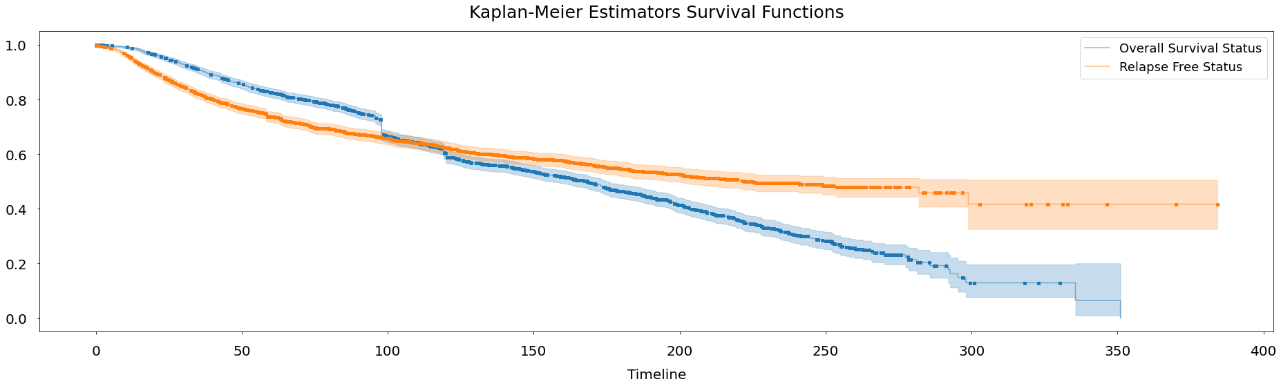

The Kaplan-meier estimate may also be used to forecast the likelihood that unobserved data will survive over time. Lifelines. KaplanMeierFitter. The times parameter of the predict function is a list of timesteps at which probabilities should be predicted. For instance, the model below aims to forecast the occurrence of both occurrences (individually) at 12, 24, and 36 months. A 5-split cross-validation and an unknown test set are used to evaluate the model.

Test ROC = 0.5 According to AUC results, the Kaplan-Meier estimate does not generalize to a new test set. Given that our model does not incorporate patient characteristics and generates identical probability for each patient in the community, this was to be expected. Because of this, Kaplan-Meier estimation is best utilized for exploratory data analysis rather than making predictions.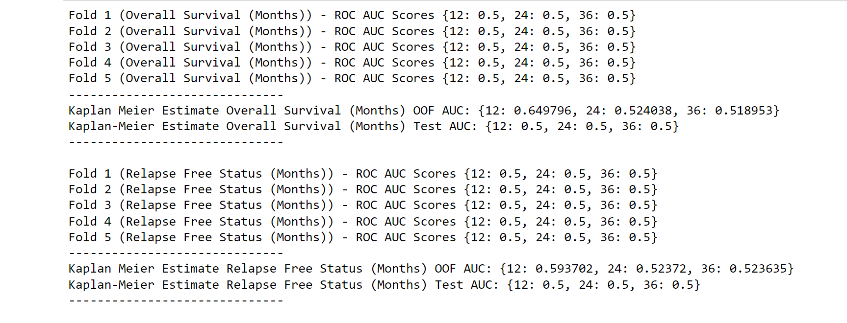

As per the result, we can see that in a year, the survival rate is 0.649796, 0.524038, and 0.518953.

Conclusion

Survival analysis using machine learning is a promising approach that can help uncover hidden patterns in the data and make more accurate predictions. While there are several challenges involved in this approach, advancements in ML techniques and computing power are making it increasingly feasible.