Working of Style Transferring

Neural style transfer is the optimization technique used to take two images- a content image and a style reference image and blend them, so the output image looks like the content image, but it "painted" in the style of the style reference image.

Import and configure the modules

Open Google colab

from __future__ import absolute_import, division, print_function, unicode_literals

try:
# %tensorflow_version only exists in Colab.
%tensorflow_version 2.x
except Exception:
pass
import tensorflow as tf

Output:

TensorFlow 2.x selected.

import IPython.display as display
import matplotlib.pyplot as plt
import matplotlib as mpl
mpl.rcParams['figure.figsize'] = (12,12)
mpl.rcParams['axes.grid'] = False
import numpy as np
import time
import functools

content_path = tf.keras.utils.get_file('nature.jpg','https://www.eadegallery.co.nz/wp-content/uploads/2019/03/626a6823-af82-432a-8d3d-d8295b1a9aed-l.jpg')
style_path = tf.keras.utils.get_file('cloud.jpg','https://i.pinimg.com/originals/11/91/4f/11914f29c6d3e9828cc5f5c2fd64cfdc.jpg')

Output:

Downloading data from https://www.eadegallery.co.nz/wp-content/uploads/2019/03/626a6823-af82-432a-8d3d-d8295b1a9aed-l.jpg
1122304/1117520 [==============================] - 1s 1us/step
Downloading data from https://i.pinimg.com/originals/11/91/4f/11914f29c6d3e9828cc5f5c2fd64cfdc.jpg
      49152/43511 [=================================] - 0s 0us/step5. def

Check the greatest measurement to 512 pixels.

load_img(path_to_img):
max_dim = 512
img = tf.io.read_file(path_to_img)
img = tf.image.decode_image(img, channels=3)
img = tf.image.convert_image_dtype(img, tf.float32)
shape = tf.cast(tf.shape(img)[:-1], tf.float32)
long_dim = max(shape)
scale = max_dim / long_dim
new_shape = tf.cast(shape * scale, tf.int32)
img = tf.image.resize(img, new_shape)
img = img[tf.newaxis, :]
return img

Creating a function to show the image

def imshow(image, title=None):
 if len(image.shape) > 3:
 image = tf.squeeze(image, axis=0)

plt.imshow(image)
if title:
plt.title(title)

content_image = load_img(content_path)
style_image = load_img(style_path)
plt.subplot(1, 2, 1)
imshow(content_image, 'Content Image')
plt.subplot(1, 2, 2)
imshow(style_image, 'Style Image')

Output: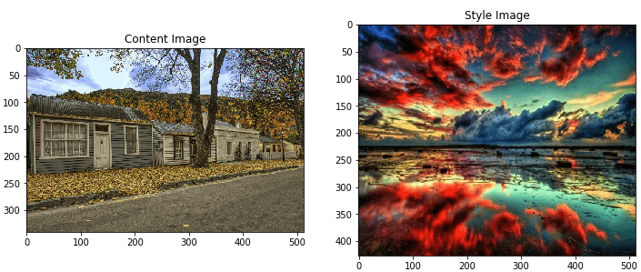

x = tf.keras.applications.vgg19.preprocess_input(content_image*255)
x = tf.image.resize(x, (224, 224))
vgg = tf.keras.applications.VGG19(include_top=True, weights='imagenet')
prediction_probabilities = vgg(x)
prediction_probabilities.shape

Output:

Downloading data from https://github.com/fchollet/deep-learning-    models/releases/download/v0.1/vgg19_weights_tf_dim_ordering_tf_kernels.h5

574717952/574710816 [==============================] - 8s 0us/step
TensorShape([1, 1000])

predicted_top_5 = tf.keras.applications.vgg19.decode_predictions(prediction_probabilities.numpy())[0]
[(class_name, prob) for (number, class_name, prob) in predicted_top_5]

Output:

Downloading data from https://storage.googleapis.com/download.tensorflow.org/data/imagenet_class_index.json
40960/35363 [==================================] - 0s 0us/step
[('mobile_home', 0.7314594),
 ('picket_fence', 0.119986326),
 ('greenhouse', 0.026051044),
 ('thatch', 0.023595566),
 ('boathouse', 0.014751049)]

Define style and content representations

Use the middle layers of the model to the content and style representation of the image. Starting from the input layer, the first few layer activation represent low-level represent like edges and textures.

For the input image, try to match the similar style and content target representation at the intermediate layers.

Load the VGG19 and run it on our image to ensure it used correctly here.

vgg = tf.keras.applications.VGG19(include_top=False, weights='imagenet')
print()
for layer in vgg.layers:
print(layer.name)

Output:

Download data from https://github.com/fchollet/deep-learning-models/releases/download/v0.1/vgg19_weights_tf_dim_ordering_tf_kernels_notop.h5
80142336/80134624 [==============================] - 2s 0us/step

input_2
block1_conv1
block1_conv2
block1_pool
block2_conv1
block2_conv2
block2_pool
block3_conv1
block3_conv2
block3_conv3
block3_conv4
block3_pool
block4_conv1
block4_conv2
block4_conv3
block4_conv4
block4_pool
block5_conv1
block5_conv2
block5_conv3
block5_conv4
block5_pool

# Content layer
content_layers = ['block5_conv2'] 

# Style layer of interest
style_layers = ['block1_conv1',
                'block2_conv1',
                'block3_conv1', 
                'block4_conv1', 
                'block5_conv1']

num_content_layers = len(content_layers)
num_style_layers = len(style_layers)

Intermediate layers for style and content

At the high level, to a network to perform image classification, it understands the image and requires taking the image as the pixels and building an internal illustration that converts the raw image pixels into a complex features present within the image.

This is also a reason why the convolutional neural networks can generalize well: they can capture the deviating and defining features within classes (e.g., cats vs. dogs) that are agnostic where the image is fed into the model and output arrangement label, the model deliver as a complex feature extractor. By accessing intermediate layers of the model, we're able to describe the style and content of input images.

Build the model

The network in tf.keras.applications are defined, so we can easily extract the intermediate layer values using the Keras functional API.

To define any model using the functional API, specify the inputs and outputs:

model= Model(inputs, outputs)

The given function builds a VGG19 model that returns a list of intermediate layer.

def vgg_layers(layer_names):
""" Creating a vgg model that returns a list of intermediate output values."""
# Load our model. Load pretrained VGG, trained on imagenet data
vgg = tf.keras.applications.VGG19(include_top=False, weights='imagenet')
vgg.trainable = False
outputs = [vgg.get_layer(name).output for name in layer_names]
model = tf.keras.Model([vgg.input], outputs)
return model

style_extractor = vgg_layers(style_layers)
style_outputs = style_extractor(style_image*255)
#Look at the statistics of each layer's output
for name, output in zip(style_layers, style_outputs):
  print(name)
  print("  shape: ", output.numpy().shape)
  print("  min: ", output.numpy().min())
  print("  max: ", output.numpy().max())
  print("  mean: ", output.numpy().mean())
  print()

Output:

block1_conv1
  shape:  (1, 427, 512, 64)
  min:  0.0
  max:  763.51953
  mean:  25.987665

block2_conv1
  shape:  (1, 213, 256, 128)
  min:  0.0
  max:  3484.3037
  mean:  134.27835

block3_conv1
  shape:  (1, 106, 128, 256)
  min:  0.0
  max:  7291.078
  mean:  143.77878

block4_conv1
  shape:  (1, 53, 64, 512)
  min:  0.0
  max:  13492.799
  mean:  530.00244

block5_conv1
  shape:  (1, 26, 32, 512)
  min:  0.0
  max:  2881.529
  mean:  40.596397

Gram matrix:

Calculating style

The content of the image is represented by the values of the common features of the map.

Calculate a Gram Matrix, which includes this information by taking the output product over all locations.

The Gram matrix can be calculated for a particular layer as: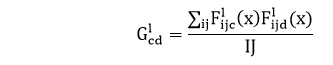

This is implemented concisely using the tf.linalg.einsum function:

def gram_matrix(input_tensor):
result = tf.linalg.einsum('bijc,bijd->bcd', input_tensor, input_tensor)
input_shape = tf.shape(input_tensor)
  num_locations = tf.cast(input_shape[1]*input_shape[2], tf.float32)
  return result/(num_locations)

Extracting the style and content of image

Building the model that returns the content and style tensor.

class StyleContentModel(tf.keras.models.Model):
def __init__(self, style_layers, content_layers):
super(StyleContentModel, self).__init__()
self.vgg =  vgg_layers(style_layers + content_layers)
self.style_layers = style_layers
self.content_layers = content_layers
self.num_style_layers = len(style_layers)
self.vgg.trainable = False
def call(self, inputs):
"Expects float input in [0,1]"
    inputs = inputs*255.0
    preprocessed_input = tf.keras.applications.vgg19.preprocess_input(inputs)
    outputs = self.vgg(preprocessed_input)
    style_outputs, content_outputs = (outputs[:self.num_style_layers],outputs[self.num_style_layers:])
style_outputs = [gram_matrix(style_output)
 for style_output in style_outputs]

    content_dict = {content_name:value for content_name, value in zip(self.content_layers, content_outputs)}
style_dict = {style_name:value
                  for style_name, value
                  in zip(self.style_layers, style_outputs)}
return {'content':content_dict, 'style':style_dict}

When called on the image, this model returns the gram matrix (style) of the style_layers and content of the content_layers:

extractor = StyleContentModel(style_layers, content_layers)
results = extractor(tf.constant(content_image))
style_results = results['style']
print('Styles:')
for name, output in sorted(results['style'].items()):
  print("  ", name)
  print("    shape: ", output.numpy().shape)
  print("    min: ", output.numpy().min())
  print("    max: ", output.numpy().max())
  print("    mean: ", output.numpy().mean())
  print()
print("Contents:")
for name, output in sorted(results['content'].items()):
  print("  ", name)
  print("    shape: ", output.numpy().shape)
  print("    min: ", output.numpy().min())
  print("    max: ", output.numpy().max())
  print("    mean: ", output.numpy().mean())

Output:

Styles:
   block1_conv1
    shape:  (1, 64, 64)
    min:  0.0055228453
    max:  28014.557
    mean:  263.79025

   block2_conv1
    shape:  (1, 128, 128)
    min:  0.0
    max:  61479.496
    mean:  9100.949

   block3_conv1
    shape:  (1, 256, 256)
    min:  0.0
    max:  545623.44
    mean:  7660.976

   block4_conv1
    shape:  (1, 512, 512)
    min:  0.0
    max:  4320502.0
    mean:  134288.84

   block5_conv1
    shape:  (1, 512, 512)
    min:  0.0
    max:  110005.37
    mean:  1487.0381

Contents:
   block5_conv2
    shape:  (1, 26, 32, 512)
    min:  0.0
    max:  2410.8796
    mean:  13.764149

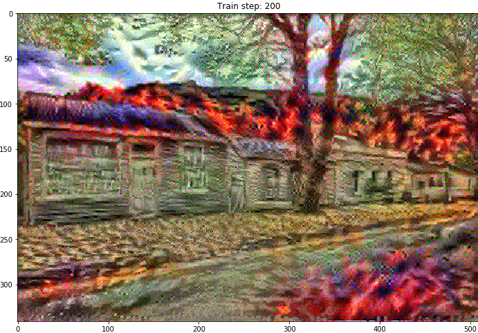
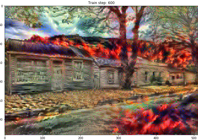
Run gradient descent

With this style and content extractor, we implement the style transfer algorithm. Do this by evaluating the mean square error in our image's output relative to each target, then take the weighted sum of the losses.

Set our style and content target values:

style_targets = extractor(style_image)['style']
content_targets = extractor(content_image)['content']

Define a tf.Variable to contain the image to hold. Initialize it with the help of content image (the tf.Variable be the same shape as the content image):

This is a floating image, define a function to keep the pixel value between 0 and 1:

def clip_0_1(image):
return tf.clip_by_value(image, clip_value_min=0.0, clip_value_max=1.0)

Create the optimizer. The paper recommends LBFGS:

To optimizing it, use a weight combination of the two losses to get the total loss:

style_weight=1e-2
content_weight=1e4

def style_content_loss(outputs):
    style_outputs = outputs['style']
    content_outputs = outputs['content']
    style_loss = tf.add_n([tf.reduce_mean((style_outputs[name]-style_targets[name])**2) 
                           for name in style_outputs.keys()])
    style_loss *= style_weight / num_style_layers

    content_loss = tf.add_n([tf.reduce_mean((content_outputs[name]-content_targets[name])**2) 
for name in content_outputs.keys()])
    content_loss *= content_weight / num_content_layers
    loss = style_loss + content_loss
    return loss

Use the function tf.GradientTape to update the image.

@tf.function()
def train_step(image):
  with tf.GradientTape() as tape:
 outputs = extractor(image)
 loss = style_content_loss(outputs)
grad = tape.gradient(loss, image)
opt.apply_gradients([(grad, image)])
  image.assign(clip_0_1(image))

Run below steps to test:

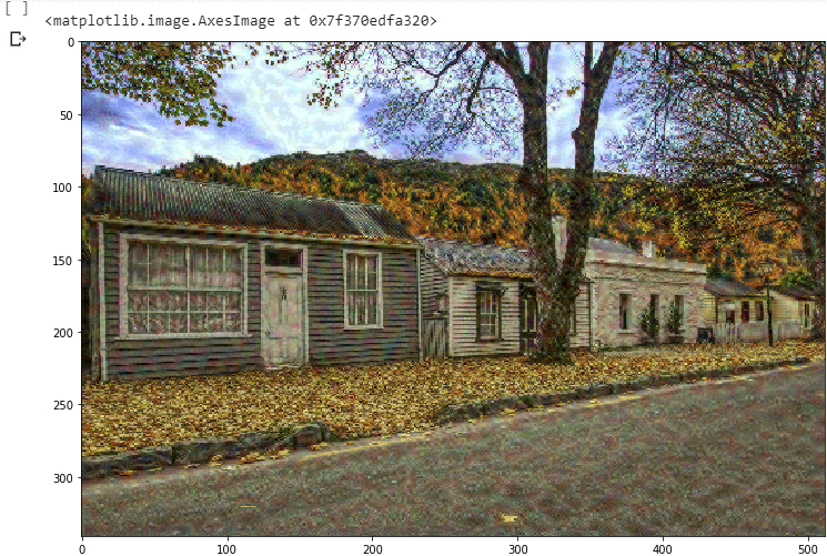
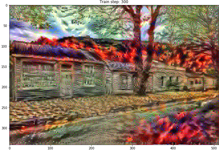
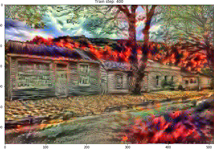
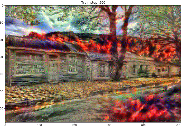
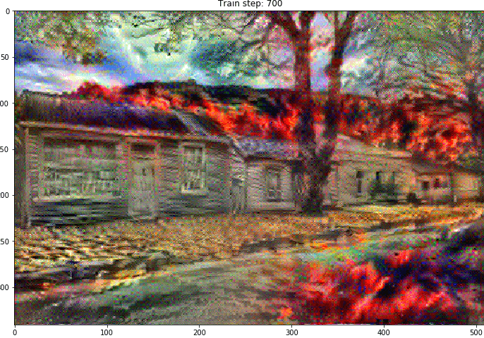
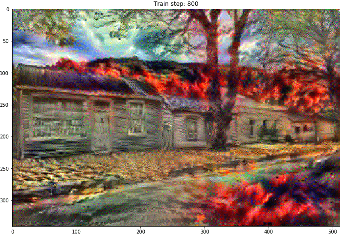
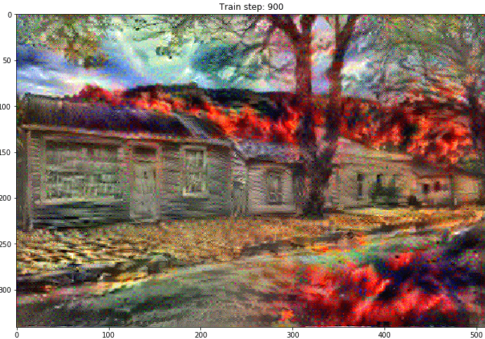
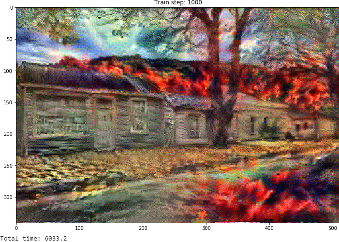
train_step (image)
train_step (image)
train_step (image)
plt.imshow(image.read_value()[0])

Output:

Transforming the image

Performing a longer optimization in this step:

import 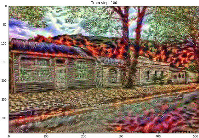time
start = time.time()

epochs = 10
steps_per_epoch = 100
step = 0
for n in range(epochs):
  for m in range(steps_per_epoch):
    step += 1
    train_step(image)
    print(".", end='')
  display.clear_output(wait=True)
  imshow(image.read_value())
  plt.title("Train step: {}".format(step))
plt.show()
end = time.time()
print("Total time: {:.1f}".format(end-start))

Output:

Total variation loss

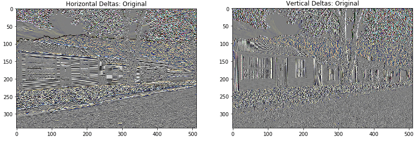
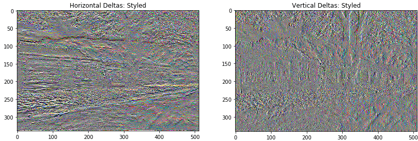
def high_pass_x_y(image):
  x_var = image[:,:,1:,:] - image[:,:,:-1,:]
  y_var = image[:,1:,:,:] - image[:,:-1,:,:]
   return x_var, y_var

x_deltas, y_deltas = high_pass_x_y(content_image)
plt.figure(figsize=(14,10))
plt.subplot(2,2,1)
imshow(clip_0_1(2*y_deltas+0.5), "Horizontal Deltas: Original")
plt.subplot(2,2,2)
imshow(clip_0_1(2*x_deltas+0.5), "Vertical Deltas: Original")
x_deltas, y_deltas = high_pass_x_y(image)
plt.subplot(2,2,3)
imshow(clip_0_1(2*y_deltas+0.5), "Horizontal Deltas: Styled")
plt.subplot(2,2,4)
imshow(clip_0_1(2*x_deltas+0.5), "Vertical Deltas: Styled")

Output:

This shows how the high frequency component have increased.

This high frequency component is an edge-detector. We get same output from the edge detector, from the given example:

plt.fig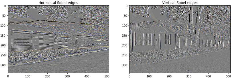ure(figsize=(14,10))
sobel = tf.image.sobel_edges(content_image)
plt.subplot(1,2,1)
imshow(clip_0_1(sobel [...,0]/4+0.5), "Horizontal Sobel-edges")
plt.subplot(1,2,2)
imshow(clip_0_1(sobel[...,1]/4+0.5), "Vertical Sobel-edges")

Output:

The regularization loss associated with this is sum of the square of the value:

def total_variation_loss(image):
  x_deltas, y_deltas = high_pass_x_y(image)
  return tf.reduce_sum(tf.abs(x_deltas)) + tf.reduce_sum(tf.abs(y_deltas))

Output:

99172.59

That demonstrate what it does. But there's no need to implement it ourselves, it includes a standard implementation:

Output:

array([99172.59], dtype=float32)

Re-running the optimization function

Pick the weight for the function total_variation_loss:

Now, train_step function:

@tf.function()
def train_step(image):
with tf.GradientTape() as tape:
outputs = extractor(image)
loss = style_content_loss(outputs)
loss += total_variation_weight*tf.image.total_variation(image)
grad = tape.gradient(loss, image)
opt.apply_gradients([(grad, image)])
image.assign(clip_0_1(image))

Reinitializing the optimization variable:

And run the optimization:

import 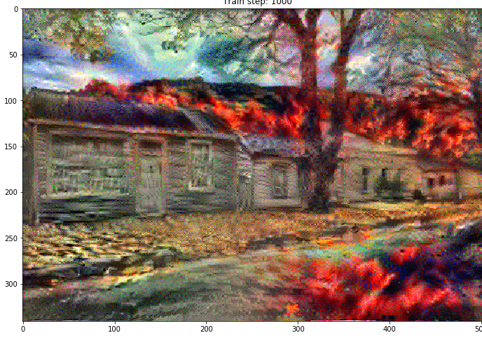time
start = time.time()

epochs = 10
steps_per_epoch = 100

step = 0
for n in range(epochs):
  for m in range(steps_per_epoch):
    step += 1
    train_step(image)
print(".", end='')
  display.clear_output(wait=True)
  display.display(tensor_to_image(image))
  print("Train step: {}".format(step))
end = time.time()
print("Total time: {:.1f}".format(end-start))

Output:

finally save the result:

file_name = 'styletransfer.png'
tensor_to_image(image). save(file_name)
try: from google. colab import files
except ImportError:
pass
else:
  files.download(file_name)

Next TopicTensorBoard

← prev next →