User-defined data structures are not inbuilt in Python, but we can still implement them. We can use the existing functional options in Python to create new data structures. For example, when we say a list = [], Python recognizes it as a list and calls everything related to a list. But when we say a linked list or a queue, Python won't know what these are. In this article, we will discuss some user-defined data structures in Python:
1. Linked Lists
A linked list, like its name suggests, is linked. Every node in the linked list consists of two segments- the data field with the data/ value and the next field holding the reference to the next node, thus linking together. It is a linear data structure, but the elements are not stored in contiguous memory locations.
Important points about Linked lists:
A linked list is an ordered collection of elements.
A linked list is also used to implement other user-defined data structures like stack and queue.
Using the collections module in Python, we can use the deque object to implement operations like insert and delete on linked lists.
The first node in a linked list is the head, and we must start all the operations on the linked list from it.
The last node of the linked list refers to None showing that the linked list is complete.
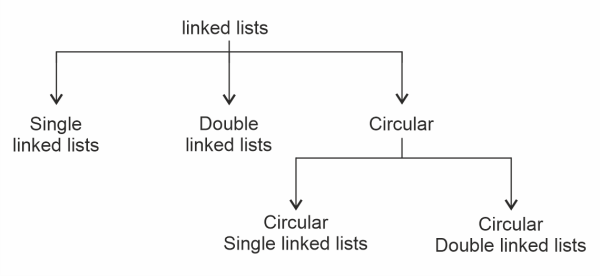
Further, linked lists are of three types:
Simple linked list
Double linked list
Circular linked list
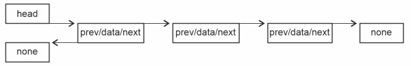
A simple linked list looks like this:
As shown in the above figure, the head is the first node, and the next (reference) part of the last node holds None.
A double-linked list looks like this:
In a double-linked list, every node will have three sections. Head holds the reference of the first node, the "previous" section of the first node holds None, and the next field of the last node refers to None. Each node will hold two references along with the data, one to its previous node and the next to the succeeding node.
Circular linked list:
A circular linked list can be single or double:
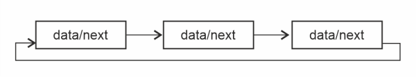
Circular single linked list:
It is a single linked list, but the last node in the list holds the reference of the first node like a circle.
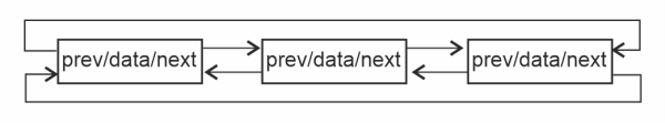
Circular double-linked list:
It is a double-linked list, but the last node in the list holds the reference of the first node, and the 'previous' section of the first node holds the reference of the last node like a circle.
Example Program:
Output:
Displaying the linked list:  10 -> 20 -> 30 -> None
Traversing from node to node:
10
20
30
After inserting 5 at the beginning: 5 -> 10 -> 20 -> 30 -> None
After inserting 40 at the end: 5 -> 10 -> 20 -> 30 -> 40 -> None
After inserting a node after 15: 5 -> 10 -> 15 -> 20 -> 30 -> 40 -> None
After inserting a node before 30: 5 -> 10 -> 15 -> 20 -> 25 -> 30 -> 40 -> None
2. Stack
Stack is a linear data structure. It is implemented on the principle "LIFO" abbreviation: Last in, first out. It means that the element that is last inserted into a stack will be the first one that gets deleted. A stack only has one opening, which means to insert or delete elements; we need to use the same end. When we insert elements into a stack, we insert elements on top of each other-new elements on the existing element. After inserting all the elements, if we want to delete elements from the stack, the last element inserted will be the first to come out.
Terminologies:
Inserting an element into the stack: push
Deleting an element from the stack: pop
The end/ opening of the stack: top of the stack
Functions in Python for stacks:
push(element)
Inserts the specified element into the stack
pop()
Deletes and returns the element at the top of the stack
top()
Returns the element at the top of the stack
peek()
Same as the top()
size()
Returns the size of the specified stack
empty()
Checks if the given stack is empty
Implementation of a stack:
We can implement a stack:
Using lists
Using linked lists
Using deque
Using queues
Output:
The elements of the stack
1
2
3
The first element to come out: 3
The second element to come out: 2
Final stack: [1]
Implementation by lists is the simplest implementation of all. To push elements into the stack, we use the list's append() method, and to pop the elements, we use the stack's pop()
Output:
Stack without pushing any elements: head None
Stack after pushing elements:
 head 14 13 12 11 10 None
After pop 3 times:
14
13
12
Stack:
 head 11 10 None
Element at the top of the stack:
11
Pop till stack becomes empty:
11
10
Traceback (most recent call last):
  File "D:\Programs\DSA \Language\Python data structures programs\stacks.py", line 59, in
    print(mystack.pop())
  File "D:\Programs\DSA\Language\Python data structures programs\stacks.py", line 34, in pop
    raise Exception("Empty stack")
Exception: Empty stack
We wrote two methods push and pop, to implement a stack. We need to make sure of two points:
When push is performed, we should always add the elements at the beginning of the linked list.
When pop is performed, the element from the beginning has to be deleted.
We created size() and isEmpty(), and top() to check if the stack is empty because if a stack is empty, we can't perform pop.
3. Queues
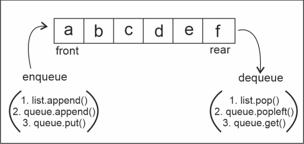
A queue is a linear data structure like a stack, but the principle of queue implementation is FIFO-First in, first out. It means that the first element inserted into the queue will be the first element to come out of the queue.
Important points about a queue:
There will be two ends to a queue-front and rear ends.
The elements are inserted from the front end and deleted from the rear end.
Terminology:
Inserting an element into a queue: enqueue
Deleting an element from the queue: dequeue
Element at the beginning: front
Element at the end: rear
We can implement a queue in Python:
Using lists
Using collections module
Using queue.Queue
Output:
Using lists:
Queue:  []
Inserting elements:
Queue: [1, 2, 3, 4, 5]
Deleting two elements:
Final queue: [3, 4, 5]

Using the deque class in the collection module
Inserting elements:
Queue: deque([6, 7, 8, 9, 10])
Deleting elements:
Final queue: deque([8, 9, 10])

Using the Queue class in the queue module
Inserting elements:
Queue:
0 1 2 3 4 5
Is the queue full? True
Deleting elements:
Final queue: [2, 3, 4, 5]
size of the queue: 4
All the inbuilt python methods used in different modules are shown above:
A queue can be related to queues in real life. The person who starts the queue gets the ticket to the movie first.
There can be a scenario of high-priority situations where irrespective of the order, we must take care of some aspects first. For such situations, there is a type of queue: Priority Queue.
Difference between Queue and Priority Queue
Regular Queue
Priority Queue
The element at the rear end is deleted when the deque operation is performed.
When the deque operation is performed, the element with the highest priority is deleted.
If two elements have the same priority, the first inserted element is deleted.
After the deque operation, the elements remain in FIFO order.
After the deque operation, the elements will either be in increasing or decreasing order.
Implementation:
Output:
Created Q: 3 2 19 90 11
Dequeue operation:
The element to be deleted: 90
Final Queue: 2 3 11 19
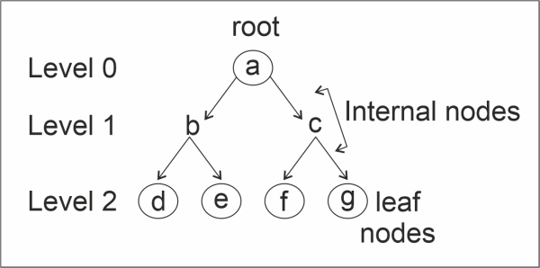
4. Binary Tree
A tree is a hierarchical representation of nodes. Family trees are real-time examples of a tree. Every node is allowed to have only two children. The node at the highest hierarchy or the top-most node is called the "Root node".
Important points about Binary tree:
Every node can have a left sub-tree and a right sub-tree.
Hence, a node in a binary tree has 3 segments: data, a reference to the left child, and a reference to the right child.
The nodes with the lowest hierarchy without any children are called leaf nodes.
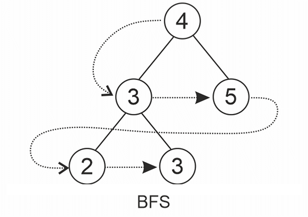
A tree can be traversed using 2 methods:
DFS: By depth
BFS: By breadth (or) level
DFS traversal further has three types of traversals:
Pre-order Traversal: The root is first visited, then the left sub-tree, followed by the right sub-tree.
Post-order Traversal: The left sub-tree is visited first, then the right sub-tree, followed by the root node.
In-order traversal: The left sub-tree is visited first, then the root node, followed by the right sub-tree.
BFS traversal is when we visit the tree level-wise.
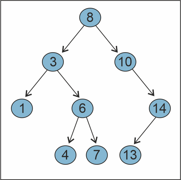
There is a type of Binary Tree called the BST or Binary Search Tree. There are three qualifications a binary tree must pass to become a BST:
The values of the nodes in the left sub-tree must be less than the value of the root node.
The values of the nodes in the right sub-tree must be greater than the value of the root node.
Every sub-tree in the tree must also follow the BST property.
Here is an example BST:
5. Graphs
In short form, G = (V, E). Here V represents vertices, and E represents edges. A graph is a non-linear Data structure. It consists of nodes/ vertices joined/ connected by edges. Both vertices and edges have to be a finite set. An edge can be represented as (u, v) given u and v are the two vertices the edge connects.
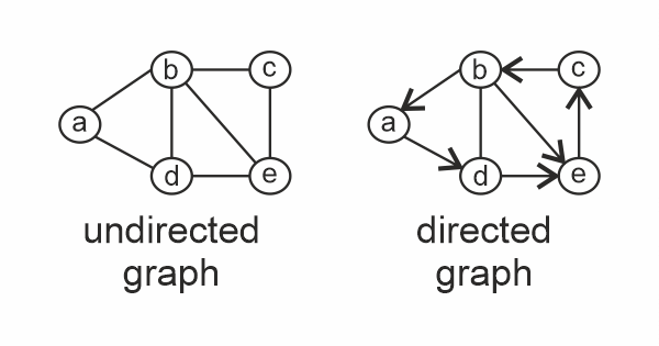
A graph can be directed or undirected. In an undirected graph, E = (u, v) and E = (v, u) are the same, while in a directed graph, they are not the same as the directed matters. Hence, edges are represented as ordered pairs of vertices the edge joins.
Important points about graphs:
The edges of a graph can have costs or weights.
Networks in real-time are represented using Graphs.
A graph can be implemented using:
Incidence matrix
Incidence List
Adjacency Matrix
Adjacency List
It is the programmer's choice of how to implement the graph based on the need in the scenario.
A graph can consist of cycles.
For graph traversal, BFS and DFS techniques are used like in trees, but to avoid visiting the same vertex again and again in the case of cycles, we need to maintain an array of visited vertices not to visit them again.
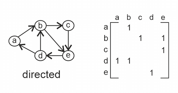
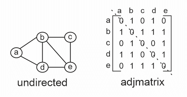
Adjacency matrix: An adjacency matrix is a (V X V) 2D array where V represents the vertices in the graph. In the matrix, adj[u][v], if in the graph, there exists an edge between u and v, adj[u][v] = 1, else 0 is assigned.
In an undirected graph, if there exists an edge from u to v, adj[u][v] = 1 and adj[v][u] = 1 as there are no directions. Hence, the adjacency matrix of an undirected graph is always symmetrical.
In a directed graph, adj[u][v] is not equivalent to adj[v][u].
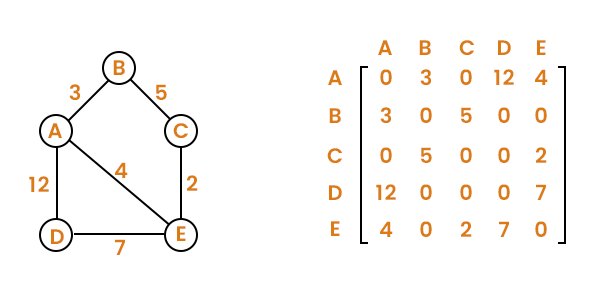
If the edges have weights are costs given, in the place of 1, we give the assigned weight/ cost in the matrix.
The disadvantage of this representation is that it takes more space-O(V2)
Here is the representation:
Here is a very simple code of adjacency matrix implementation for the graph:
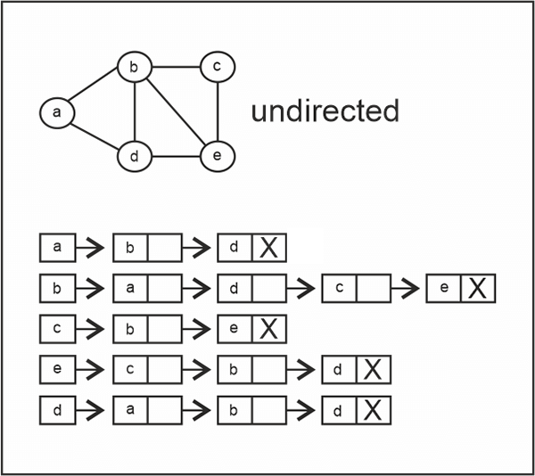
To implement an adjacency list, we use an array/ list of linked lists to represent the vertices and edges in the graph. The number of linked lists used in the representation equals the number of vertices in the graph.
An array with length = no-of vertices is created, and for every vertex, we will create a linked list with all the adjacent vertices, and these linked lists will be arranged in the array.
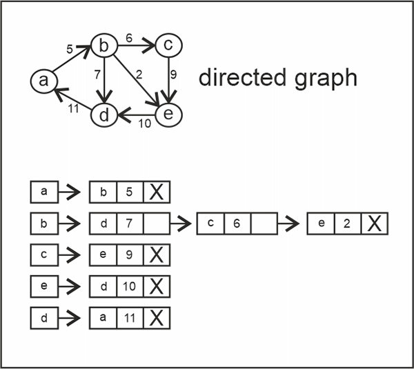
In the case of a directed graph, all the nodes/ vertices we can travel to from the node in the array are linked in the linked list.
Simple, an adjacency list is an array of linked lists with adjacent nodes of the first node.
Here is the representation:
In the above adjacency list representation, the graph is undirected. Hence, each node's neighboring nodes in the graph are linked as separate linked lists.
This is a directed graph. Hence, for each node in the graph, adjacent/ neighboring nodes that we can direct from the node are linked.
Also, costs are given to every edge in the graph. Hence, the costs are also represented in the linked lists.
Here is a simple code with an adjacency list representation of a graph:
A list of the size number of vertices in the graph is created with all None values:
[None, None, None, None, None]
Now, when an edge(source, destination) call is made:
Using the class node, a destination node is created, and its next is pointed to the source in the array, and then the linked list is assigned to the source position in the array.


 For Videos Join Our Youtube Channel: Join Now