Define Beam Search

Beam search is a heuristic search algorithm that explores a graph by expanding the most optimistic node in a limited set. Beam search is an optimization of best-first search that reduces its memory requirements.

Best-first search is a graph search that orders all partial solutions according to some heuristic. But in beam search, only a predetermined number of best partial solutions are kept as candidates. Therefore, it is a greedy algorithm.

Beam search uses breadth-first search to build its search tree. At each level of the tree, it generates all successors of the states at the current level, sorting them in increasing order of heuristic cost. However, it only stores a predetermined number (β), of best states at each level called the beamwidth. Only those states are expanded next.

The greater the beam width, the fewer states are pruned. No states are pruned with infinite beam width, and beam search is identical to breadth-first search. The beamwidth bounds the memory required to perform the search. Since a goal state could potentially be pruned, beam search sacrifices completeness (the guarantee that an algorithm will terminate with a solution if one exists). Beam search is not optimal, which means there is no guarantee that it will find the best solution.

In general, beam search returns the first solution found. Once reaching the configured maximum search depth (i.e., translation length), the algorithm will evaluate the solutions found during a search at various depths and return the best one that has the highest probability.

The beam width can either be fixed or variable. One approach that uses a variable beam width starts with the width at a minimum. If no solution is found, the beam is widened, and the procedure is repeated.

Components of Beam Search

A beam search takes three components as its input:

1. A problem to be solved,
2. A set of heuristic rules for pruning,
3. And a memory with a limited available capacity.

The problem is the problem to be solved, usually represented as a graph, and contains a set of nodes in which one or more of the nodes represents a goal. The set of heuristic rules are rules specific to the problem domain and prune unfavorable nodes from memory regarding the problem domain.

The memory is where the "beam" is stored, memory is full, and a node is to be added to the beam, the most costly node will be deleted, such that the memory limit is not exceeded.

Beam Search Algorithm

The following algorithm for a beam search, as a modified best-first search, is adapted from Zhang's 1999:

Uses of Beam Search

A beam search is most often used to maintain tractability in large systems with insufficient memory to store the entire search tree. For example,

• It has been used in many machine translation systems.
• Each part is processed to select the best translation, and many different ways of translating the words appear.
• According to their sentence structures, the top best translations are kept, and the rest are discarded. The translator then evaluates the translations according to a given criterion, choosing the translation which best keeps the goals.
• The first use of a beam search was in the Harpy Speech Recognition System, CMU 1976.

Drawbacks of Beam Search

Here is a drawback of the Beam Search with an example:

• In general, the Beam Search Algorithm is not complete. Despite these disadvantages, beam search has found success in the practical areas of speech recognition, vision, planning, and machine learning.
• The main disadvantages of a beam search are that the search may not result in an optimal goal and may not even reach a goal at all after given unlimited time and memory when there is a path from the start node to the goal node.
• The beam search algorithm terminates for two cases: a required goal node is reached, or a goal node is not reached, and there are no nodes left to be explored.
• A more accurate heuristic function and a larger beam width can improve Beam Search's chances of finding the goal.

For example, let's take the value of ß = 2 for the tree shown below. So, follow the following steps to find the goal node.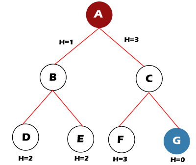

Step 1: OPEN= {A}

Step 2: OPEN= {B, C}

Step 3: OPEN= {D, E}

Step 4: OPEN= {E}

Step 5: OPEN= { }

The open set becomes empty without finding the goal node.

NOTE: But with the value of ß = 3, the algorithm succeeds in finding the goal node.

Beam Search Optimality

The Beam Search algorithm is not complete in some cases. Therefore it is also not guaranteed to be optimal. It can happen because of these reasons:

• The beam width and an inaccurate heuristic function may cause the algorithm to miss expanding the shortest path.
• A more precise heuristic function and a larger beam width can make Beam Search more likely to find the optimal path to the goal.

For example, we have a tree with heuristic values shown below: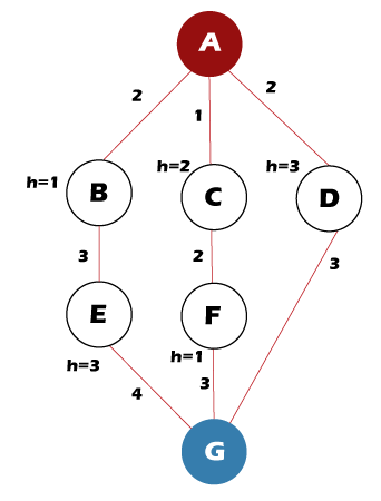

Follow the following steps to find the path for the goal node.

Step 1: OPEN= {A}

Step 2: OPEN= {B, C}

Step 3: OPEN= {C, E}

Step 4: OPEN= {F, E}

Step 5: OPEN= {G, E}

Step 6: Found the goal node {G}, now stop.

Path: A-> C-> F-> G

But the Optimal Path is A-> D-> G

Time Complexity of Beam Search

The time complexity of the Beam Search algorithm depends on the following things, such as:

• The accuracy of the heuristic function.
• In the worst case, the heuristic function leads Beam Search to the deepest level in the search tree.
• The worst-case time = O(B*m)

B is the beam width, and m is the maximum depth of any path in the search tree.

Space Complexity of Beam Search

The space complexity of the Beam Search algorithm depends on the following things, such as:

• Beam Search's memory consumption is its most desirable trait.
• Since the algorithm only stores B nodes at each level in the search tree.
• The worst-case space complexity = O(B*m)

B is the beam width, and m is the maximum depth of any path in the search tree.

• This linear memory consumption allows Beam Search to probe very deeply into large search spaces and potentially find solutions that other algorithms cannot reach.

Variants of Beam Search

Beam search has been made complete by combining it with depth-first search, resulting in beam stack search and depth-first beam search. With limited discrepancy search, beam search results in limited discrepancy backtracking (BULB).

The resulting search algorithms are anytime algorithms that find reasonable but likely sub-optimal solutions quickly, like beam search, then backtrack and continue to find improved solutions until convergence to an optimal solution.

In the context of a local search, we call local beam search a specific algorithm that begins selecting β generated states. Then, for each level of the search tree, it always considers β new states among all the possible successors of the current ones until it reaches a goal.

Since local beam search often ends up on local maxima, a standard solution is to choose the next β states in a random way, with a probability dependent on the heuristic evaluation of the states. This kind of search is called stochastic beam search.

Other variants are flexible beam search and recovery beam search.