MIRROR OF MATRIX ACROSS DIAGONAL

Introduction

The concept of mirroring a matrix across its slant, frequently referred to as slant mirroring or reflection across the slant, is an abecedarian operation in direct algebra and mathematics. This operation involves transubstantiating a matrix in such a way that it becomes symmetric with respect to its main slant, creating a glass image of the original matrix. Slant mirroring has wide operations in fields such as matrix factorization, eigenvalue calculations, and optimization problems. It plays a pivotal role in simplifying matrix parcels and operations. This operation is important for theoretical understanding and also for practical operations in data analysis, signal processing, and colorful scientific disciplines. In this environment, we will explore the principles and ways behind mirroring a matrix across its slant and claw into its significance in mathematics and its practical mileage in solving real-world problems. Understanding slant mirroring is essential for a deeper appreciation of matrix operations and their operations in different disciplines.

Given a 2-D array of order N x N, publish a matrix that's the glass of the given tree across the slant. We need to publish the result in a way that exchanges the values of the triangle above the slant with the values of the triangle below it, like a glass image exchange. Publish the 2-D array attained in a matrix layout.

Properties of mirror matrix across diagonal

Reflecting a matrix across its slant, also known as slant mirroring or reflection across the slant, has several parcels and counteraccusations in direct algebra and colorful fine operations. Then, there are some of the crucial parcels associated with this operation.

The result of mirroring a matrix across its slant is a symmetric matrix. This means that the matrix is equal to its transpose, and the rudiments on either side of the slant are glass images of each other.
Eigenvalues Diagonal mirroring doesn't alter the eigenvalues of the original matrix. However, if the original matrix has eigenvalues λ_1 λ_n, the imaged matrix will also have the same eigenvalues.
Orthogonality is the process of slant mirroring. It is orthogonal, conserving the fleck product of vectors. However, the fleck product( xT) *(y) is the same as the fleck product( yT) *(x) for the imaged matrix if you have vectors x and y.
Real-Symmetric Matrices Diagonal mirroring is particularly applicable for real symmetric matrices, where the eigenvalues are real and the eigenvectors are orthogonal. This operation retains the real symmetric property.
Eigenvalue Decomposition For real symmetric matrices, slant mirroring can be seen as an orthogonal metamorphosis that diagonalizes the matrix by transforming it into a slant matrix. This process is basic for working with colorful fine problems, including eigenvalue corruption.
Simplification Slant mirroring simplifies matrix computations and allows for easier calculation of matrix powers and exponentials, as the imaged matrix retains the same eigenvalues and orthogonal eigenvectors.
operations Slant mirroring is extensively used in fields like quantity mechanics, amount computing, drugs, and statistics, where the parcels of real symmetric matrices are essential.
Invariance Diagonal mirroring is an isometric operation, meaning it preserves distances and angles between vectors. This property is precious in operations where geometric metamorphoses need to be maintained.

Implementation

A simple result of this problem involves redundant space. We cut each right diagonal (right-to-left wing) one by one. During the traversal of the slant, first, we push all the rudiments into the mound, then we cut it again and replace every element of the slant with the mound element.

The basic program for the implementation of the mirror matrix across the diagonal is as follows:

# Simple or basic program for implementing the mirror of a matrix using Python.
m = 100
def MM (matrix, size):
# For the diagonal of a matrix, which starts at the first row of the matrix.
r = 0
# Traversing of the right diagonal of the matrix.
for j in range(size):
# Stack is used here for reversing the elements of the matrix.
s = []
i = r
k = j
while (i < size and k >= 0):
s.append(matrix[i][k])
i += 1
k -= 1
# Pushing all the elements of the matrix into a stack in reverse order.
i = r
k = j
while (i < size and k >= 0):
matrix[i][k] = s[-1]
k -= 1
i += 1
s.pop()
# Doing the same process for the diagonals that start at the end of each column.
c = size - 1
for j in range (1, size): 
# The stack is used for reversing the elements here;
s = []
i = j
k = c
while (i < size and k >= 0):
s.append(matrix[i][k])
i += 1
k -= 1
# Pushing all the elements of the matrix into a stack in reverse order.
i = j
k = c
while (i < size and k >= 0):
matrix[i][k] = s[-1]
i += 1
k -= 1
s.pop()
# Function defined for the printing of the matrices.
def PM (matrix, size):
for i in range(size):
for j in range(size):
print(matrix[i][j], end=" ")
print()
# The driver code or the main code.
matrix = [[1, 2, 3, 4], [5, 6, 7, 8],
[9, 10, 11, 12], [13, 14, 15, 16]]
size = 4
print ("The matrix given is")
PM (matrix, size)
print ("The mirror matrix of the given matrix across the diagonal is:")
MM (matrix, size)
PM (matrix, size)

Output:

The output of the program that is written above is given as follows: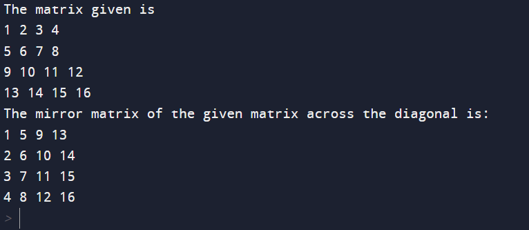

Time complexity O(n2)

Auxiliary Space O(n), as mound is used.

Explanation of the code:

The handed Python law glasses a square matrix across its main slant. Then, there is a detailed explanation of the law.

The law starts by defining a function called MM (mirror matrix) and another function called PM (publish matrix) for matrix operations and printing independently. The motorist law initializes a sample 4x4 matrix and prints it.

The MM serves as the input matrix across its main slant. It does this in two corridors.

Top-left to bottom-right inclinations: It iterates through the inclinations starting from the top-left corner (row 0, column 0) to the bottom-right corner (row size 1, column size 1). For each slant, it uses a mound to reverse the rudiments' order along that slant. It pushes the slanted rudiments onto the mound and pops them back into the matrix in reverse order. This operation is done for all similar inclinations.
**Top-right to bottom-left inclinations** Also, it processes the inclinations starting from the top-right corner (row 0, column size 1) to the bottom-left corner (row size 1, column 0). It uses the same mound-ground reversal fashion for these inclinations.

After calling the MM function, the law prints the imaged matrix using the PM function. The result is a matrix where the rows have been reversed, effectively creating a glass image of the original matrix across its main slant.

In the illustration given, the law glasses the original 4x4 matrix, and the final imaged matrix is published, showing the metamorphosis across the main slant.

Method -2

Observing a matrix with output reveals a successful fix for this issue: all we need to do is switch (mat[i][j] to mat[j][i]).

The issues with the above program are resolved using the technique given below.

An effective way to apply a glass matrix in Python is to produce a new matrix by switching rows and columns of the original matrix using list appreciation. Then is how you can do it compactly and effectively.

python
def mirror_matrix( matrix):
    mirrored_matrix = ((matrix (j)( i) for j in range( len (matrix))) for i in range( len (matrix)))
    returnmirrored_matrix

This law iterates through the rows and columns of the original matrix, switching them to induce the imaged matrix. It runs in O (n2) time, where 'n' is the size of the matrix, making it an effective and terse result for creating a glass image of the input matrix across its main slant.

# For finding the mirror of the matrix across the diagonal, the effective way is defined as follows.
from builtins import range
M = 100; 
def MM (matrix, size): 
# Traversing the matrix and swapping the elements. 
for i in range(size): 
for j in range (i + 1):
t = matrix[i][j]; 
matrix[i][j] = matrix[j][i] 
matrix[j][i] = t 
# The function used for printing the matrix. 
def PM (matrix, size): 
for i in range(size): 
for j in range(size): 
print(matrix[i][j], end=" "); 
print(); 
# The driver code or the primary code is as follows. 
if __name__ == '__main__': 
matrix = [1, 2, 3, 4], [5, 6, 7, 8], [9, 10, 11, 12], [13, 14, 15, 16]; 
size = 4; 
print("The matrix that is to be processed or that is to be changed for mirror matrix:") 
print(matrix)
print("The matrix that is changed or the mirror matrix after the implementation of the program is:")
MM (matrix, size); 
PM (matrix, size); 

Output:

The output of the program that is written above is given as follows: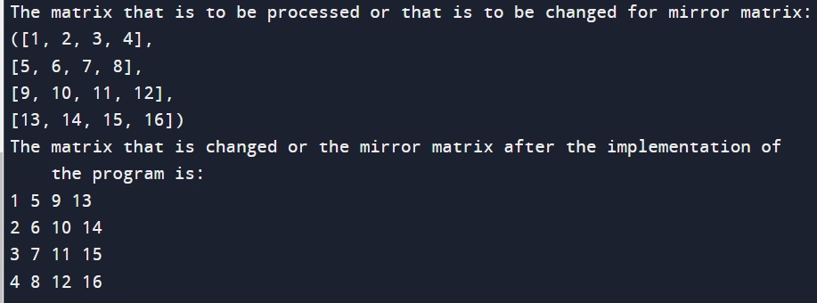

Explanation of the code

This Python law defines a program to find the glass matrix of a given square matrix. The MM function takes a matrix and its size as parameters, and it traverses the upper triangle of the matrix, switching rudiments across the main slant. This switching effectively transposes the matrix, resulting in its glass image. The PM function is responsible for publishing the matrix rudiments in a readable format.

In the main section (if name == ', main,'), a 4x4 matrix named matrix is initialized, and its original form is published. The glass matrix is also attained by calling the MM function, and both the original and glass matrix are published using the PM function.

The matrix is represented as a list of lists, where each inner list corresponds to a row of the matrix. The use of the range function facilitates replication over matrix indicators.

Overall, the law demonstrates a simple matrix manipulation operation, furnishing a clear illustration of the process of carrying a glass matrix through transposition. It serves as an educational illustration for understanding nested circles, matrix manipulation, and the basics of Python programming.

Complexities of the above code.

The law has a time complexity of O(n2) due to nested circles for matrix transposition and printing. The space complexity is O(n2), substantially lower than storing the input matrix as a list of lists. Temporary variables have constant space. Overall, the law efficiently finds the glass matrix, demonstrating quadratic time and space complexity, where n is the size of the square matrix.

Conclusion

In summary, the Python law efficiently computes the glass matrix of a square matrix by switching rudiments across its main slant. The time complexity of the transposition operation is O (n2), with n being the matrix size due to nested circles. The space complexity is also O (n2), as the matrix is represented as a list of lists. The law provides a terse and instructional illustration of matrix manipulation, illustrating the process of carrying a glass image. It's particularly beneficial for learners as it demonstrates abecedarian generalities similar to nested circles, matrix traversal, and transposition in Python. Overall, this law is a precious resource for those seeking to understand and apply matrix metamorphoses across the main slant.

Next TopicPair of strings having longest common prefix of maximum length in given array

← prev next →