Sort an almost sorted array

Introduction

Sorting algorithms are essential to data manipulation and computer science. Although there are many different sorting algorithms available, each one's effectiveness is dependent on the properties of the data that needs to be sorted. Sorting an almost-sorted array, in which each element is at most k positions from its sorted position, is an intriguing scenario. An almost sorted array is a special case in which the elements are somewhat, but not quite, in the order in which they were sorted. Each element is at most k positions away from its final sorted position, which is a crucial feature. When compared to generic sorting techniques, this property enables more efficient sorting algorithms.

Insertion Sort

The Insertion Sort technique is one of the most straightforward and effective sorting algorithms available, especially when used to sort an almost-sorted array, which is a unique situation. This algorithm works by gradually adding each element to the final sorted array one at a time. The array's separation into a sorted and an unsorted subarray is crucial to its efficacy. As it moves through the unsorted section, the algorithm compares each element and moves it into the appropriate spot in the sorted subarray. When dealing with nearly sorted arrays where every element is at most k positions from its sorted position, this procedure is especially helpful.

By taking advantage of the current order and reducing the number of comparisons and swaps that are required, the Insertion Sort algorithm performs well in this situation. While O(n^2)'s worst-case time complexity could seem like a disadvantage, it's actually a useful and practical option because of how well it handles small datasets and partially ordered datasets. By restricting the movement of elements, indicated by the parameter k, Insertion Sort effectively converts an almost sorted array into its fully ordered counterpart, demonstrating the adaptability and potency of the algorithm in particular sorting situations.

Code

Output:

Code Explanation

Function Declaration

• The required header file is included at the beginning of the program, and the insertionSort function is declared. Three parameters are required for this function: the size of the array n, the maximum displacement k, and an integer array arr.

Logic for Insertion Sort

• The insertionSort function, which performs the actual sorting, is the brain of the program. It adheres to the Insertion Sort algorithm, which loops over the array beginning with element two (i = 1).
• It compares each element with those in the sorted subarray (i.e., elements that come before the current position).
• To make room for the current element, an element in the sorted subarray that is larger than the current element is shifted to the right.
• This procedure is repeated until the current element in the sorted subarray is located at the proper location and inserted there.

Main Function

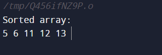
• An example array arr is declared and initialized with values {12, 11, 13, 5, 6} in the main function.
• To provide flexibility in the event that the array size changes, the sizeof the operator is used to calculate the size of the array n.
• Three is the maximum displacement k that is set.
• After that, the array, its size, and the maximum displacement are passed as arguments to the insertionSort function.

Printing the Sorted Array

• The sorted array is printed to the console in the main function via a straightforward loop once the sorting process is finished.

Output

• The sorted array that results from the program's final run shows how well the Insertion Sort algorithm sorts the provided almost-sorted array.

Time Complexity

• Worst Case: The worst-case scenario, which happens when the array is arranged in reverse order and each element needs to be compared and moved to the proper location, is O(n^2).
• Best Case: O(n) - This happens when there is already some sorting of the array and very little or no element shifting is needed.

Space Complexity

• O(1): Insertion Since sort is an in-place sorting algorithm, its temporary variables are kept in a constant amount of additional memory. More space is not needed in proportion to the size of the input.

Heap Sort

One popular sorting algorithm that works well in situations where elements are nearly sorted inside an array is heap sort. The binary heap, a specialized tree-based data structure, is a concept that the algorithm makes use of. Heap Sort excels at rearranging data quickly when applied to an almost sorted array, where each element is at most k positions from its sorted position. The heapification and sorting phases make up the two main stages of the algorithm. The array is converted into a max-heap during heapification, guaranteeing that every parent node is greater than or equal to each of its children.

Following the establishment of the max-heap, the sorting step entails decreasing the heap size, regaining the max-heap property, and repeatedly switching the root, or maximum element, with the last element. Until the entire array is sorted, this process is repeated. Large datasets can benefit from Heap Sort's O(n * log(n)) time complexity, which contributes to its efficiency. Its ability to take advantage of the current order demonstrates its adaptability to nearly sorted arrays, producing a reliable sorting algorithm for a range of situations.

Code

Output:

Code Explanation

Header Files

• The code contains the required header files, <stdlib.h> for dynamic memory allocation and other utility functions, and <stdio.h> for input and output operations.

heapify Function

• It is the function's responsibility to keep the max-heap property intact.
• The array arr, its size n, and the index i, which indicates the subtree root, are its three required parameters.
• The function finds the largest child and the root by identifying the left (l) and right (r) offspring of the current node.
• It switches the elements and recursively calls heapify on the impacted subtree if the largest is not the root.

heapSort Function

• The primary purpose of Heap Sort. The array arr, its size n, and the maximum displacement k are the three parameters required.
• Constructing a max-heap from the input array is the first step. Every time iterating from the final non-leaf node to the root, the loop calls heapify.
• The second stage starts after the max-heap has been constructed. The heap size is decreased by exchanging the last element with the largest element (at the root).
• Then, in order to preserve the max-heap property, heapify is called on the root. Until the entire array is sorted, this process is repeated.

main Function

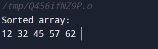
• An example array arr is declared and initialized with values {12, 32, 45, 57, 62} in the main function.
• To provide flexibility in the event that the array size changes, the sizeof the operator is used to calculate the size of the array n.
• Three is the maximum displacement k that is set.
• Next, the array, its size, and the maximum displacement are passed as arguments to the heapSort function.

Printing the Sorted Array

• The sorted array is printed to the console in the main function via a straightforward loop once the sorting process is finished.

Output

• The sorted array, which displays how well the Heap Sort algorithm sorted the input array, is the program's final output.

Time Complexity

• Worst Case: O(n log n) - Heap Sort is effective for handling big datasets because its time complexity is consistently O(n log n) in all scenarios.
• Best Case: O(n log n) - Heap Sort works well in situations where consistency in performance is crucial because the best-case time complexity is equal to the worst-case time complexity.

Space Complexity

• O(1) - Heap Since sort is an in-place sorting algorithm, it continuously uses additional memory for variables. More space is not needed in proportion to the size of the input.

Merge Sort

Merge Sort is a very effective method, particularly when arranging an almost sorted array. Using a divide-and-conquer tactic, this algorithm divides the array into smaller parts, sorts each part separately, and then combines them to create the final ordered array. The fundamental idea behind Merge Sort is its capacity to handle nearly sorted arrays, in which every element is at most k positions from its sorted position. Merge Sort reduces the effect of displacement by splitting the array into smaller pieces, enabling a more efficient sorting procedure. An essential part of the algorithm is the merge function, which cleverly combines two sorted arrays into a single sorted array.

This approach works well for nearly sorted arrays because it preserves the current order and minimizes the total number of comparisons and moves. Merge Sort is effective for sorting large datasets because of its time complexity of O(n log n). Still, it is also important in sorting scenarios where there are particular pre-ordering constraints because of its flexibility in responding to the peculiarities of almost sorted arrays. Merge Sort is a dependable option for sorting nearly sorted arrays due to its systematic approach and efficiency with partially ordered datasets, demonstrating the algorithm's adaptability and efficacy.

Code

Output:

Code Explanation

Header Files and Function Declarations

• The two functions merge and mergeSort are declared after the program includes the required header files, <stdio.h> and <stdlib.h>.

Merge Function

• An essential component of the Merge Sort algorithm is the merge function. The array arr, the indices l (left), m (middle), and r (right) are its four required parameters.
• It determines the sizes of L and R, the two subarrays that need to be merged.
• The data from the original array is copied into temporary arrays L and R, which are then created.
• Subsequently, the function combines the two temporary arrays into the original array, sorting them accordingly.

Merge Sort Function

• The primary recursive function that carries out the Merge Sort algorithm is the mergeSort function.
• The array arr and the indices l (left), m (middle), and r (right) are its four required parameters.
• When l is less than r, the recursion's base case signifies that the subarray contains at least two elements.
• To split the array in half, the function finds the middle index or m.
• For both the left and right sides of the array, recursive calls to mergeSort are made.
• Lastly, the sorted halves are merged by calling the merge function.

Main Function

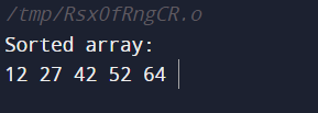
• An example array arr is declared and configured with values {12, 27, 42, 52, 64} in the main function.
• The sizeof operator is used to determine the size of the array n.
• Three is the maximum displacement k that is set.
• Next, the array, its size, and the maximum displacement are passed as arguments to the mergeSort function.

The Sorted Array is printed

• The sorted array is printed to the console in the main function via a straightforward loop once the sorting process is finished.

Output

• The sorted array, which shows how well the Merge Sort algorithm sorted the input array, is the program's final output.

Time Complexity

• Worst Case: O(n log n) - Merge Sort is effective for large datasets because it consistently displays a time complexity of O(n log n) for all scenarios.
• Best Case: O(n log n) - Merge Sort works well in situations where consistency in performance is crucial because its best-case time complexity is equal to that of the worst-case.

Space Complexity

O(n) - Combination The space complexity of the sort is directly related to the size of the input array. In order to create temporary arrays during the merging process, more memory is needed. Comparing the space complexity to in-place sorting algorithms such as Insertion Sort and Heap Sort is less optimal.