Warshall's Algorithm

Warshall's algorithm is used to determine the transitive closure of a directed graph or all paths in a directed graph by using the adjacency matrix. For this, it generates a sequence of n matrices. Where, n is used to describe the number of vertices.

R(0), ..., R(k-1), R(k), ... , R(n)

A sequence of vertices is used to define a path in a simple graph. In the k^th matrix (R^(k)), (r_ij^(k)), the element's definition at the i^th row and j^th column will be one if it contains a path from v_i to v_j. For all intermediate vertices, w_q is among the first k vertices that mean 1 ≤ q ≤ k.

The R⁽⁰⁾ matrix is used to describe the path without any intermediate vertices. So we can say that it is an adjacency matrix. The R⁽ⁿ⁾ matrix will contain ones if it contains a path between vertices with intermediate vertices from any of the n vertices of a graph. So we can say that it is a transitive closure.

Now we will assume a case in which r_ij^(k) is 1 and r_ij^(k-1) is 0. This condition will be true only if it contains a path from v_i to v_j using the v_k. More specifically, the list of vertices is in the following form

vi, wq (where 1 ≤ q < k), vk. wq (where 1 ≤ q < k), vj 

The above case will be occur only if r_ik^(k-1) = r_kj^(k-1) = 1. Here, k is subscript.

The r_ij^(k) will be one if and only if r_ij^(k-1) = 1.

So in summary, we can say that

rij(k) = rij(k-1) or (rik(k-1) and rkj(k-1))

Now we will describe the algorithm of Warshall's Algorithm for computing transitive closure

Warshall(A[1...n, 1...n]) // A is the adjacency matrix
R(0) ← A
for k ← 1 to n do
for i ← 1 to n do
for j ← to n do
R(k)[i, j] ← R(k-1)[i, j] or (R(k-1)[i, k] and R(k-1)[k, j])
return R(n)

Here,

• Time efficiency of this algorithm is (n³)
• In the Space efficiency of this algorithm, the matrices can be written over their predecessors.
• Θ(n³) is the worst-case cost. We should know that the brute force algorithm is better than Warshall's algorithm. In fact, the brute force algorithm is also faster for a space graph.

Example of Transitive closure

In this example, we will consider two graphs. The first graph is described as follows: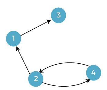

The matrix of this graph is described as follows: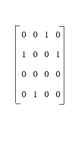

The second graph is described as follows: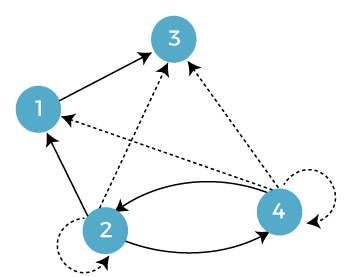

The matrix of this graph is described as follows: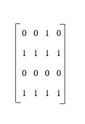

The main idea of these graphs is described as follows:

• The vertices i, j will be contained a path if
• The graph contains an edge from i to j; or
• The graph contains a path from i to j with the help of vertex 1; or
• The graph contains a path from i to j with the help of vertex 1 and/or vertex 2; or
• The graph contains a path from i to j with the help of vertex 1, 2, and/or vertex 3; or
• The graph contains a path from i to j with the help of any other vertices.

On the kth iteration, the algorithm will use the vertices among 1, …., k, known as the intermediate, and find out that there is a path exists between i and j vertices or not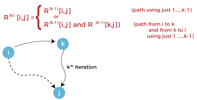

In a directed graph, the transitive closure with n vertices is used to describe the n-by-n Boolean matrix T. Where, elements in the ith row and jth column will be 1. This can occur only if it contains a directed path form ith vertex to jth vertex. Otherwise, the element will be zero. The transitive closure is described as follows: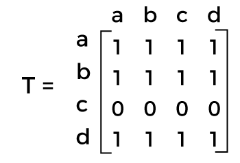

The adjacency matrix is a type of square matrix, which is used to represent a finite graph. In the graph, the element of a matrix is used to indicate whether pairs of vertices are adjacent or not. The adjacency matrix can also be known as the connection matrix, which has rows and columns. A simple labeled graph with the position 0 or 1 will be represented by the rows and columns. The position of 0 or 1 will be assigned in a graph on the basis of condition the whether Vi and Vj are adjacent or not. If the graph contains an edge between two nodes, then it will assign as 1. If the graph has no nodes, then it will assign as 0. The adjacency matrix is described as follows: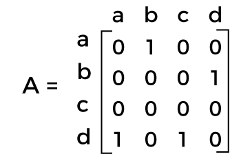

A digraph is a pair of characters. The digraph is described as follows: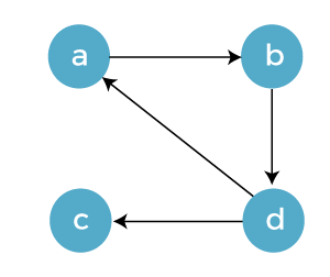

Warshall's Algorithm (Matrix generation)

Recurrence relating elements R(k) to elements of R(k-1) can be described as follows:

R(k)[i, j] = R(k-1)[i, j] or (R(k-1)[i, k] and R(k-1)[k, j])

In order to generate R(k) from R(k-1), the following rules will be implemented:

Rule 1: In row i and column j, if the element is 1 in R(k-1), then in R(k), it will also remain 1.

Rule 2: In row i and column j, if the element is 0 in R(k-1), then the element in R(k) will be changed to 1 iff the element in its column j and row k, and the element in row i and column k are both 1's in R(k-1).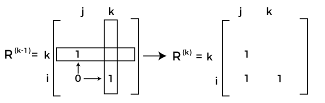

Application of Warshall's algorithm to the directed graph

In order to understand this, we will use a graph, which is described as follow:

For this graph R(0) will be looked like this: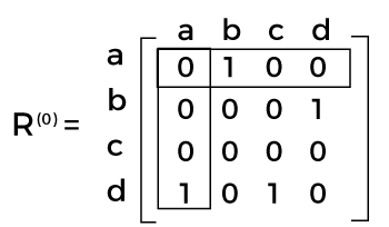

Here R(0) shows the adjacency matrix. In R(0), we can see the existence of a path, which has no intermediate vertices. We will get R(1) with the help of a boxed row and column in R(0).

In R(1), we can see the existence of a path, which has intermediate vertices. The number of the vertices is not greater than 1, which means just a vertex. It contains a new path from d to b. We will get R(2) with the help of a boxed row and column in R(1).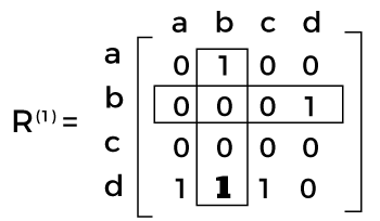

In R(2), we can see the existence of a path, which has intermediate vertices. The number of the vertices is not greater than 2, which means a and b. It contains two new paths. We will get R(3) with the help of a boxed row and column in R(2).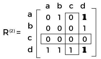

In R(3), we can see the existence of a path, which has intermediate vertices. The number of the vertices is not greater than 3, which means a, b and c. It does not contain any new paths. We will get R(4) with the help of a boxed row and column in R(3).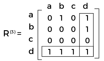

In R(4), we can see the existence of a path, which has intermediate vertices. The number of the vertices is not greater than 4, which means a, b, c and d. It contains five new paths.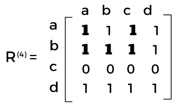

Example 1:

In this example, we will assume A = {1, 2, 3, 4} and let R be the relation on A whose matrix is described as follows: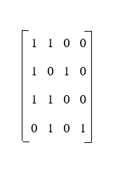

Now we will use Warshall's algorithm to compute M_R∞.

Solution:

Here, matrix is the starting point. So matrix is described as follows: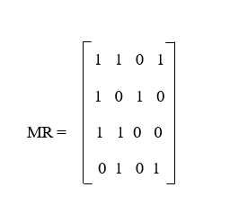

Now we will assume W₀ = M_R and then successively compute W₁, W₂, W₃, and W₄. (If we have an M_R which contains n * n matrix, in this case, we will assume W₀ = W_R and compute W₁, W₂, W₃, …., W_n.) For each k>0, Wk is calculated with the help of row k and column k of W_k-1. So we can say that W₁ is computed with the help of column 1 and row 1 of W₀ = M_R, W₂ is calculated with the help of column 2 and row 2 of W₁, and the same process will be followed for W₃, W₄, and so on. The step by step process to get W_k from W_k-1 is described as follow:

Step 1:

In this step, we will transfer all 1's in W_k-1 to the corresponding position of W_k. If we take k = 1 for this problem, then we get the following table: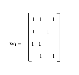

Step 2:

Now we will make of list separately of all the columns that have 1's in row k and all the rows that have 1's in column k. After separation, we will get columns 1, 2, and 4, and rows 1, 2, and 3.

Step 3:

In this step, we will pair each of the row numbers with each of the column numbers. If there is not 1 in the paired position, then we will add 1 in that position of W₁. In all the empty positions, we will put 0.

The pairs which we get are described as follow:

(1, 1), (1, 2), (1, 4), (2, 1), (2, 2), (2, 4), (3, 1), (3, 2) and (3, 4).

The matrix with the help of these pairs is described as follows: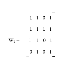

Now we will repeat the same process for k = 2. The first step will provide us the following matrix: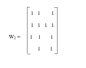

Using the second step, we will get the row numbers 1, 2, 3, 4 and column numbers 1, 2, 3, 4. With the help of third step, we will get all possible pairs of row numbers and column numbers for k = 2, which are described as follows:

(1, 1), (1, 2), (1, 3), (1, 4), (2, 1), (2, 2), (2, 3), (2, 4), (3, 1), (3, 2), (3, 3), (3, 4), (4, 1), (4, 2), (4, 3), and (4, 4).

The matrix with the help of these pairs is described as follows: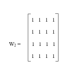

In this example, we will also have to calculate W₃ and W₄, but we know that W₃ and W₄ will get the same result as W₂. According to this algorithm, if an entry in Wk-1 is 1, then the entry of Wk will remain the same as 1. Hence in Wk+1, …, Wn.

Thus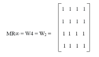

And the transition closure R can be defined as the total relation A*A, which contains every possible ordered pair of elements of A. So it can specify that everything in A is related by

R^∞ to everything in A.

Now we will use the Boolean operation ∧ and ∨ on {0, 1} so that we can understand this algorithm more formally. If Wij(k) is the (i, j) entry of Wk, then on the basis of the above-described steps, we can say that

wij(k) = w(k?1)ij ∨ (w(k?1)ik ∧ w(k?1)kj) 

According to the second step of this algorithm, if i exists in the row list and j exists in the column list, then w(k?1)ik∧w(k?1)kj=1will be 1. If the third step of this algorithm either shows w_ij^(k) was already 1, which shows in the first step, or (i, j) is one of the pairs formed in the third step.