Hashing - Open Addressing for Collision Handling

We have talked about

• A well-known search method is hashing.
• When the new key's hash value matches an already-occupied bucket in the hash table, there is a collision.

Open Addressing for Collision Handling

Similar to separate chaining, open addressing is a technique for dealing with collisions. In Open Addressing, the hash table alone houses all of the elements. The size of the table must therefore always be more than or equal to the total number of keys at all times (Note that we can increase table size by copying old data if needed). This strategy is often referred to as closed hashing. The foundation of this entire process is probing. We will comprehend several forms of probing later.

• Insert (k): Continue probing until a slot is left open. Put k in the first empty spot you find.
• Search (k): Continue probing until either an empty slot is found or the slot's key no longer equals k.
• Delete (k): An intriguing delete procedure. The search can fail if we just remove a key. Therefore, deleted key slots are specifically noted as "deleted."

Although an item can be inserted into a deleted slot, the search continues after the slot has been empty.

NOTE-

• The "removed" buckets are handled the same as any other empty buckets during insertion.
• When searching, the search does not stop when it comes across a "deleted" bucket.
• Only when the necessary key or an empty bucket are discovered does the quest come to an end.

Open Addressing

Open addressing is when

• All the keys are kept inside the hash table, unlike separate chaining.
• The hash table contains the only key information.

The methods for open addressing are as follows:

• Linear Probing
• Quadratic Probing
• Double Hashing

The following techniques are used for open addressing:

(a) Linear probing

In linear probing, the hash table is systematically examined beginning at the hash's initial point. If the site we receive is already occupied, we look for a different one.

The rehashing function is as follows: table-size = (n+1)% rehash(key). As may be seen in the sample below, the usual space between two probes is 1.

Let S be the size of the table and let hash(x) be the slot index calculated using a hash algorithm.

Let's use "key mod 7" as a simple hash function with the following keys: 50, 700, 76, 85, 92, 73, 101.

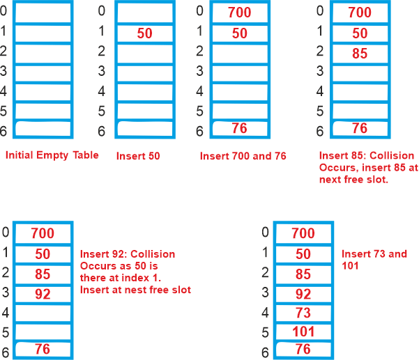
Linear probing problems:

• Primary Clustering: Primary clustering is one of the issues with linear probing. Many successive items form clusters, making it difficult to locate a free slot or to search for an element.
• Secondary Clustering: Secondary clustering is less severe, and two records can only share a collision chain (also known as a probe sequence) if they start out in the same location.

Advantage-

• Calculating this is simple.

Disadvantage-

• Clustering is the fundamental issue with linear probing.
• Groups are composed of several adjacent pieces.
• After then, searching for an element or an empty bucket takes time.

Time Complexity:

The worst time in linear probing to search an element is O ( table size ). This is due to

• even if all other elements are absent and there is only one element.
• The hash table's "deleted" markers then force a full table search.

(b) Quadratic probing

If you pay close attention, you will notice that the hash value will cause the interval between probes to grow. The above-discussed clustering issue can be resolved with the aid of the quadratic probing technique. The mid-square method is another name for this approach. We search for the i2'th slot in the i'th iteration using this strategy. We always begin where the hash was generated. We check the other slots if only the location is taken.

c) Double Hash

Another hash function calculates the gaps that exist between the probes. Clustering is optimally reduced by the use of double hashing. This method uses a different hash function to generate the increments for the probing sequence. We search for the slot i*hash2(x) in the i'th rotation using another hash algorithm, hash2(x).

Comparing the first three:

• The best cache performance is provided by linear probing, although clustering is a problem. Linear probing also has the benefit of being simple to compute.
• Between the two in terms of clustering and cache performance is quadratic probing.
• Although double hashing lacks clustering, it performs poorly in caches. Due to the necessity to compute two hash functions, double hashing takes longer to compute.

Because we traverse a Linked List by essentially jumping from one node to the next throughout the computer's memory, chaining's cache efficiency is poor. Because of this, the CPU is unable to cache nodes that haven't been visited yet, which is bad for us. However, since data isn't dispersed while using Open Addressing, the CPU can cache information for speedy access if it notices that a particular area of memory is frequently accessed.

Performance of Open Addressing: Similar to Chaining, the performance of hashing can be assessed assuming that each key has an equal likelihood of being hashed to any slot of the table (simple uniform hashing)

Load Factor (α)-

Load factor (α) is defined as-

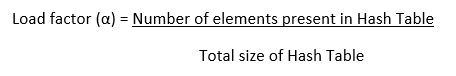
The load factor value in open addressing is always between 0 and 1. This is due to

• In open addressing, the hash table contains all of the keys.
• As a result, the table's size is always more than or at least equal to the number of keys it stores.

Conclusions-

• The best cache performance is achieved via linear probing, although clustering is a problem.
• Between the two in terms of clustering and cache performance is quadratic probing.
• Although clustering is absent, double caching has poor cache performance.