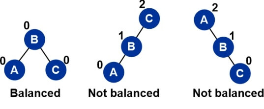
Properties of AVL Trees

In 1962, GM Adelson-Velsky and EM Landis created the AVL Tree. To honors the people who created it, the tree is known as AVL.

The definition of an AVL tree is a height-balanced binary search tree in which each node has a balance factor that is determined by deducting the height of the node's right sub tree from the height of its left sub tree.

If each node's balance factor falls between -1 and 1, the tree is considered to be balanced; otherwise, the tree needs to be balanced.

Balance Factor

• The left sub-tree is one level higher than the right sub-tree if the balancing factor of any node is 1.
• Any node with a balance factor of zero indicates that the heights of the left and right sub trees are equal.
• If a node's balancing factor is negative one, the left sub-tree is one level behind the right sub-tree.
• In the following figure, an AVL tree is presented. We can observe that each node's associated balancing factor ranges from -1 to +1. So, it is an illustration of an AVL tree.
• We're going to talk about AVL trees today and how they're used. The worst-case performance of BST is shown to be closest to that of linear search algorithms, i.e. O (n). We are unable to forecast data patterns and frequencies in real-time data. Therefore, the necessity to balance out the current BST emerges.
• AVL trees, which stand for Adelson, Velski, and Landis, are height-balancing binary search trees. The AVL tree ensures that the height difference between the left and right sub-trees is no greater than 1. Balance Factor is the name for this.
• To better grasp the distinction between balanced and unbalanced trees, let's look at some examples:
  

• Because the height to the left and right of the root node is the same in the example above, we can see that the first tree is balanced. While the other two are not like that, the tree in the middle picture is lopsided to the left of the node. In a similar manner, the tree is lopsided to the right of the root node in the last image on the right, rendering it imbalanced.

Why use AVL Trees?

The majority of BST operations, including search, max, min, insert, delete, and others, require O(h) time, where h is the BST's height. For a skewed Binary tree, the cost of these operations can increase to O(n). We can provide an upper bound of O(log(n)) for all of these operations if we make sure that the height of the tree stays O(log(n)) after each insertion and deletion. An AVL tree's height is always O(log(n)), where n is the tree's node count.

Operations on AVL Trees

Due to the fact that, AVL tree is also a binary search tree hence, all the operations are conducted in the same way as they are performed in a binary search tree. Searching and traversing do not lead to the violation in property of AVL tree. However, the actions that potentially break this condition are insertion and deletion; as a result, they need to be reviewed.

• Insertion
• Deletion

Insertion in AVL Trees

We must add some rebalancing to the typical BST insert procedure to ensure that the provided tree stays AVL after each insertion.

The following two simple operations (keys (left) key(root) keys(right)) can be used to balance a BST without going against the BST property.

• Rotate left
• Rotate right

The steps to take for insertion are:

• Let w be the newly added node.
• carry out a typical BST insert for w.
• Find the first imbalanced node by moving up starting at w. Assume that z is the initial imbalanced node, y is z's kid who arrives on the path from w to z, and x is z's grandchild that arrives on the aforementioned path.
• Rotate the z-rooted subtree in the proper directions to rebalance the tree. As x, y, and z can be ordered in 4 different ways, there may be 4 potential scenarios that need to be addressed.
• The four potential configurations are as follows:
  • Left Left Case: y is z's left child and x's left child.
  • Left Right Case: z's right child and x's right child.
  • Right Right Case: y is z's right child and x's left child.
  • Right Right Case: y is z's right child and x's left child.

The procedures to be carried out in the four circumstances indicated above are listed below. In every instance, we only need to rebalance the subtree rooted with z, and the entire tree will be balanced as soon as the height of the subtree rooted with z equals its pre-insertion value (with the proper rotations).

1. Left Left Case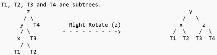

2. Left Right Case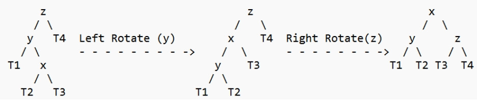

3. Right Right Case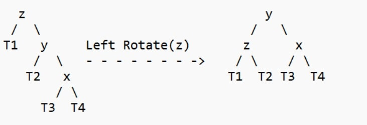

4. Right Left Case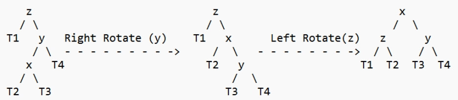

Advantages of AVL Trees

• The AVL tree's height never exceeds log N, where N is the total number of nodes in the tree, since the height is always balanced.
• When compared to straightforward Binary Search trees, it provides a superior search time complexity.
• AVL trees are capable of self-balancing.

Disadvantages of AVL Trees

• The aforementioned examples show that AVL trees can be challenging to implement.
• Additionally, for particular operations, AVL trees have significant constant factors.
• Red-black trees, as opposed to AVL trees, are used in the majority of STL implementations of the ordered associative containers (sets, multisets, maps, and multimaps). Red-black trees, unlike AVL trees, only need one restructure for an insertion or removal.

AVL trees, which were developed specifically to balance imbalanced binary trees used in database indexing, can be said to have served a specific purpose. The only difference between them and binary search trees is that in this case, we need to maintain the balance factor, which means that the data structure should remain a balanced tree as a result of various operations, which are accomplished by using the AVL tree Rotations that we previously learned about.

Properties of AVL Tree

Property 1: The most number of nodes an AVL tree of height H might have

= 2^H+1 - 1

Maximum possible number of nodes in AVL tree of height-3

= 23+1 - 1

= 16 - 1

= 15

Thus, in AVL tree of height-3, maximum number of nodes that can be inserted = 15

Property 2: A recursive relation determines the minimum number of nodes in an AVL Tree of height H.

N(H) = N(H-1) + N(H-2) + 1

Base conditions for this recursive relation are-

N(0) = 1

N(1) = 2

Property 3: The AVL Tree's smallest feasible height with N nodes

= [log2N]

Minimum possible height of AVL Tree using 8 nodes

= [log28]

= [log223]

= [3log22]

= [3]

= 3

Property 4: Using recursive relation, the maximum height of an AVL tree with N nodes is computed.

N(H) = N(H-1) + N(H-2) + 1

Base conditions for this recursive relation are-

N(0) = 1

N(1) = 2

NOTE:

• The maximum height of an AVL Tree with n nodes cannot be greater than 1.44log2n.
• In other words, 1.44log2n is the worst-case height of an AVL tree with n nodes.

Problems on AVL Trees

Problem 1: Find the bare minimum of nodes needed to build an AVL tree with height = 3.

Solution- As is well known, a recursive relation determines the least number of nodes in an AVL tree of height H.

N(H) = N(H-1) + N(H-2) + 1

where N(0) = 1 and N(1) = 2

Step-01:

Substituting H = 3 in the recursive relation, we get-

N(3) = N(3-1) + N(3-2) + 1

N(3) = N(2) + N(1) + 1

N(3) = N(2) + 2 + 1 (Using base condition)

N(3) = N(2) + 3 …………(1)

To solve this recursive relation, we need the value of N(2).

Step-02:

Substituting H = 2 in the recursive relation, we get-

N(2) = N(2-1) + N(2-2) + 1

N(2) = N(1) + N(0) + 1

N(2) = 2 + 1 + 1 (Using base conditions)

∴ N(2) = 4 …………(2)

Step-03:

Using (2) in (1), we get-

N(3) = 4 + 3

∴ N(3) = 7

Thus, minimum number of nodes required to construct AVL tree of height-3 = 7.