Self-Balancing Binary Search Trees

Data Structures are a specified way to organize and store data in computers in such a manner that we can execute operations on the stored data more effectively and efficiently. Binary Search Trees (BSTs) are vital in performing efficient operations among the different data structures available.

In the following tutorial, we will learn about the Self-Balancing Binary Search Tree, a data structure that evades a few drawbacks of the standard Binary Search Tree by confining its height.

So, let's get started.

Understanding the Binary Search Trees

A Binary Search Tree (abbreviated as BST) is a special type of Binary Tree where the value of the data element at each node is greater than or equal to all node values in its left sub-tree and less than or equal to all node values in its right sub-tree.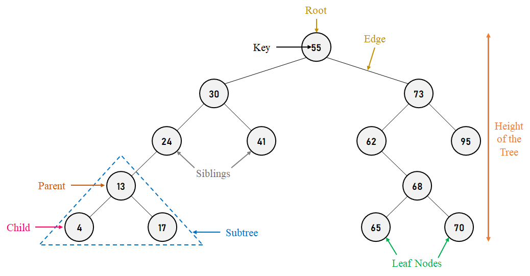

Figure 1. Visualization of Basic Terminology of Binary Search Trees

Let us now have a look at some of the key terms associated with Binary Search Tree:

1. A leaf is a node having no children.
2. The number of nodes on the path from the root node down to (and including) that specific node is known as the depth of a node.
3. The maximum depth of a binary tree refers to the depth of its deepest left. Thus, we can also consider it as the height of the tree.
4. A Tree is said to be balanced if, for every node in the tree, the height of its left and right sub-trees differs by at most 1.

Operations of the Binary Search Tree

A Binary Search Tree generally supports operations like Insertion, Deletion, and Searching. The Time complexity of each operation depends upon the height of the tree, which means that the operation will have to traverse all the nodes present on the path from the root to the deepest leaf in the worst case.

Let us consider a problem as an example where the tree is heavily skewed. A figure demonstrating the same is shown below: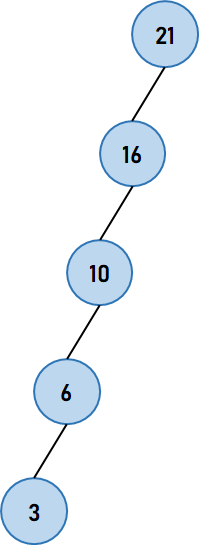

Figure 2. A Heavily Skewed Tree

Although the tree shown in the above figure is a valid Binary Search Tree, it is ineffective. If we want to insert, search, or delete a node from the above tree, we may be traversing every node present.

Thus, the worst-case time complexity of each operation on the above tree is O(n), where n is the number of nodes in the tree.

However, we are aiming for a balanced tree.

A balanced tree is a tree where, for every node, the height of its left and right sub-trees differs by, at most 1. Therefore, the height of a balanced binary tree is bounded by O(log₂?n), which means that each operation will have the time complexity of O(log₂?n) in the worst case. We can think of it as an important improvement from O(n).

Understanding the Self-Balanced Binary Search Tree

One way to ensure that the tree is always balanced is by the implementation of a Self-Balancing Binary Search Tree. A Self-Balancing Binary Search Tree is a Binary Search Tree (BST) that inevitably attempts always to maintain its height to a minimum, ensuring that its operations will maintain a worst-case time complexity of O(log₂?n).

Let us understand the above statement mathematically for better knowledge.

A Binary Tree with height h can have at most 2⁰ + 2¹ + 2² + ... + 2^h = 2^(h+1) - 1 nodes.

n ≤ 2^h+1 -1

h ≥ ⌈log_2?(n + 1) - 1 ⌉ ≥ ⌊log_2? n ⌋

Hence, with respect to the Self-Balancing Binary Search Trees, the minimum height must be equal to the floor value of log_2? n. Moreover, a binary tree is said to be balanced if the height of left and right sub-trees of every node differs by either -1, 0, or + 1. This value is called the Balance Factor.

Balance Factor

= Height of the Left Subtree-Height of Right Subtree

How do Self-Balancing Binary Search Trees balance?

Regarding self-balancing, Binary Search Trees perform rotations after the execution of an insert and delete operations. The following are the two types of rotation operations that can be performed to balance the Binary Search Trees without breaching the property of the Binary Search Tree:

1. Left Rotation
2. Right Rotation

Let us now understand the above two operations in brief.

Left Rotation

The Left Rotation is one of the operations of the Binary Search Tree where we push a node, N, down to the left in order to balance the tree. This rotation assumes that node N has the right child (or sub-tree). The right child, R, of node N, becomes the parent node of N, and the left child of R becomes the new right child of node N. This rotation is used specifically when the right sub-tree of node N has a considerably (depending on the tree's type) greater height than its left sub-tree.

Let us now consider the following figure illustrating the same.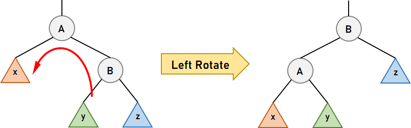

Figure 3. Left Rotation of node A

In the above figure, when we left rotate about node A, node B becomes the new root of the subtree. Node A becomes the left child of node B, and the sub-tree, y, becomes the right child of node A.

Right Rotation

The Right Rotation is another operation of the Binary Search Tree where we push a node, N, down to the right in order to balance the tree. This rotation assumes that node N has a left child (or sub-tree). The left child, L, of the node N, becomes the parent node of N, and the right child of L becomes N's new left child. This rotation is specifically used when the left sub-tree of node N has a considerably (depending on the tree's type) greater height than its right sub-tree.

Let us now consider the following figure illustrating the same.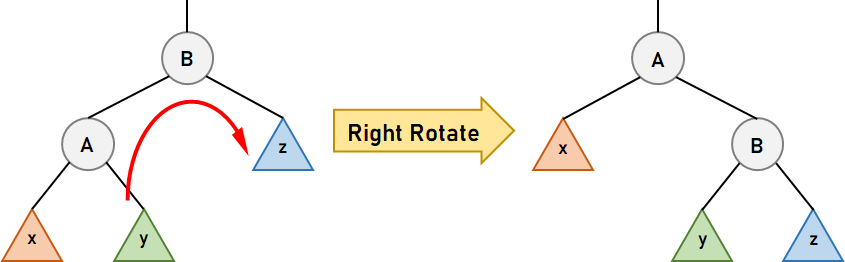

Figure 4. Right Rotation of Node B

In the above figure, when we right rotate about node B, node A becomes the new root of the subtree. Node B becomes the left child of node A, and the sub-tree, y, becomes the left child of node A.

Note:

Once the rotations are done, the in-order traversal of nodes in both the previous and final trees will be the same, and the Binary Search Tree property will retain.

Understanding the Types of Self-Balancing Binary Search Trees

The following are some data structures that implement this type of Tree:

1. 2-3 Tree
2. Red-Black Tree
3. AA Tree
4. AVL Tree
5. B Tree
6. Scapegoat Tree
7. Splay Tree
8. Tango Tree
9. Treap
10. Weight Balanced Trees

Let us now discuss these trees in brief.

2-3 Tree

A 2-3 Tree is a Self-Balancing Binary Search Tree where each node in the tree has either:

1. Two Children and a Data Element, or
2. Three Children and two Data Elements, or
3. Leaf nodes are at the same level having no child but either one or two Data Elements.

Let us consider an example of a 2-3 Tree: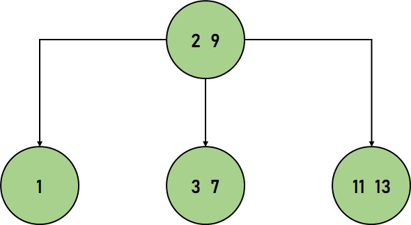

Figure 5. A 2-3 Tree

From the above figure, we can observe that this tree satisfies all the rules mentioned earlier.

The Time Complexity in Big-O notation for a 2-3 Tree for the average and worst case is the same, i.e.,

1. Space - O(?n)
2. Search - O(log₂?n)
3. Insert - O(log₂?n)
4. Delete - O(log₂?n)

Red-Black Tree

A Red-Black Tree is a Self-Balancing Binary Search Tree where each node stores an additional bit representing the color used to ensure the balancing of the tree during the insertion and deletion operations. Every node of this Tree must follow the following rules, including the ones imposed by a Binary Search Tree:

1. Every node is colored either Black or Red.
2. The Roots of the Tree is always Black.
3. All the leaves of the Tree that are NIL must be Black.
4. No Two Red nodes should be adjacent, meaning that a red node can neither have a red child nor a red parent.
5. Every path from a node to its descendant NIL nodes has the same number of Black nodes.

The following is an example of the Red-Black Tree: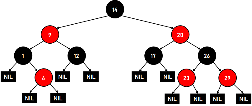

Figure 6. A Red-Black Tree

The Time Complexity in Big-O notation for a Red-Black Tree for the average and worst case is the same, i.e.,

1. Space - O(?n)
2. Search - O(log₂?n)
3. Insert - O(log₂?n)
4. Delete - O(log₂?n)

AA Tree

The AA Tree is the variation of the Red-Black Trees, which uses the concept of levels in order to balance Binary Trees. However, in contrast to the Red-Black Trees, the Red nodes on an AA Tree can only be added as a right child, which also means that the Red nodes cannot be present as a left child. The AA Trees follow the following five rules:

1. The Level of every leaf node in an AA Tree is one.
2. The Level of every left child is precisely one less than that of its parent.
3. The Level of every right child is less than or equal to that of its parent.
4. The Level of every right grandchild is strictly less than that of its grandparent.
5. Every node of a Level greater than one has two children.

The following is an example of an AA Tree: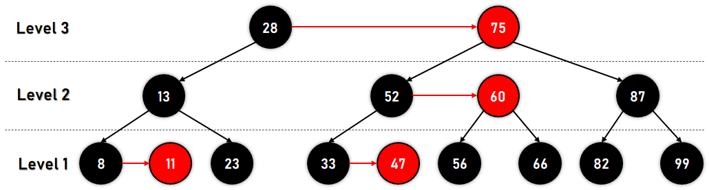

Figure 7. An AA Tree

The AA Tree guarantees fast operations with time complexity of ? (log₂?n), and its implementation code is the shortest among all the balanced trees.

AVL Tree

The AVL Tree is another example of a Self-Balancing Binary Search Tree where the difference between the heights of the left and right subtrees can't be more than one for all the nodes present in the Tree. This difference is also known as the Balance Factor and is defined as:

Balance Factor

= Height of the Left Subtree-Height of Right Subtree

The Balance Factor for an AVL Tree is an integer ranging from -1 to 1.

The following is an example of an AVL Tree: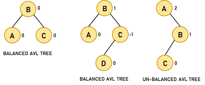

Figure 8. An AVL Tree

The Time Complexity in Big-O notation for an AVL Tree in the worst case is as follows:

1. Space - O(?n)
2. Search - O(log₂?n)
3. Insert - O(log₂?n)
4. Delete - O(log₂?n)

B-Tree

A B-Tree is another example of the Self-Balancing Binary Search Tree, which simplifies the Binary Search Tree, allowing the nodes with more than two children.

As per the definition of Knuth, a B-Tree of order m is a tree that satisfies some properties as follows:

1. Every node of a B-Tree has at most n children.
2. Every non-leaf node (except root) has at least [n/2] child nodes.
3. If the root is not a leaf node, it has at least two children.
4. A non-leaf node with m children consists of m - 1 keys.
5. All leaves exist at the same level and carry no information.

Let us consider the following example of a B-Tree: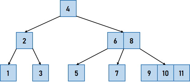

Figure 9. A B-Tree

B-Trees are well suited for storage systems that read and write a reasonably large block of data. These Trees are also used in databases and file systems.

Important Point: A B-Tree of order 3 is considered as a 2-3 Tree.

The Time Complexity in Big-O notation for a B-Tree for the average and worst case is the same, i.e.,

1. Space - O(?n)
2. Search - O(log₂?n)
3. Insert - O(log₂?n)
4. Delete - O(log₂?n)

Scapegoat Tree

A Scapegoat Tree is a type of Self-Balancing Binary Search Tree that does not require any additional storage for every node of the tree. The Scapegoat Tree becomes an attractive choice as a Self-Balancing Binary Search Tree due to the low overhead and easy implementation.

The balancing concept is to ensure that the nodes are α (alpha) size balanced, which implies that the size of the left and right sub-tress are at most α times the node's size, i.e., α � (node's size). This idea is on the basis of the fact that if a node is α weight balanced, it is also height balanced, having the height less than or equal to log_(1/α) size + 1..

The Time Complexity in Big-O notation for a Scapegoat Tree for the average case is as follows:

1. Space - O(?n)
2. Search - O(log₂?n)
3. Insert - O(log₂?n)
4. Delete - O(log₂?n)

The Time Complexity in Big-O notation for a Scapegoat Tree for the worst case is as follows:

1. Space - O(?n)
2. Search - O(log n)
3. Insert - Amortized O(log n)
4. Delete - Amortized O(log n)

Splay Tree

A Splay Tree is another example of the Self-Balancing Binary Search Tree where the tree has an additional property for accessing the recently accessed elements quickly again. This tree consists of all the operations of a Binary Search Tree, like insertion, deletion, and search, with the inclusion of one more operation known as Splaying. Splaying is a common operation in a Splay Tree involved with every operation performed at the root of the tree. Splaying of the Tree for a certain data element rearranges the tree so that the data element is placed at its root.

For example, whenever we perform a standard Binary Search for a particular data element, followed by the rotations of a tree in a particular order such that this data element is placed as the root. We could also use a Top-Down algorithm to combine the search and reorganization operations into a single phase.

Splaying depends upon three factors while accessing a data element (for example, x):

1. Whether the data element, x, is the left or right child of its parent node, p.
2. Whether the parent node, p, is the root or not, and if not.
3. Whether the parent node, p, is the left or right child of its parent, q (the grandparent of x).

On the basis of the above factors, we have categorized the rotations into different types:

1. Zig Rotation [Right Rotation]
2. Zig Zig Rotation [Two Right Rotation]
3. Zag Rotation [Left Rotation]
4. Zag Zag Rotation [Two Left Rotation]
5. Zig Zag Rotation [Zig followed by Zag]
6. Zag Zig Rotation [Zag followed by Zig]

The Time Complexity in Big-O notation for a Splay Tree for the average case is as follows:

1. Space - O(?n)
2. Search - O(log n)
3. Insert - O(log n)
4. Delete - O(log n)

The Time Complexity in Big-O notation for a Splay Tree for the worst case is as follows:

1. Space - O(?n)
2. Search - Amortized O(log n)
3. Insert - Amortized O(log n)
4. Delete - Amortized O(log n)

Treap

The Treap data structure is a type of Self-Balancing Binary Search Tree and a combination of both a Binary Tree and a Binary Tree; however, it does not promise a height of O(log₂ n). The idea is to utilize randomization and binary heap property in order to maintain the high probability balance.

Every node of a Treap consists of two values:

1. KEY: The Key is a value that follows standard Binary Search Tree ordering.
2. PRIORITY: The Priority is a randomly assigned value that follows the max-heap property.

Let us consider the following example of a Treap: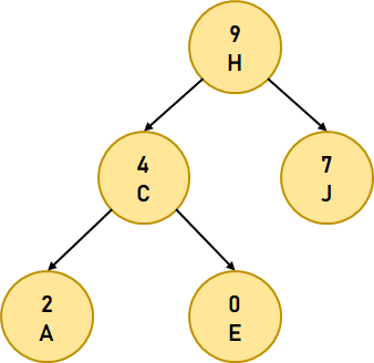

Figure 10. A Treap

The above figure exemplifies a Treap with an alphabetic key and numeric max heap order.

The Time Complexity in Big-O notation for a Treap for the average case is as follows:

1. Space - O(?n)
2. Search - O(log₂?n)
3. Insert - O(log₂?n)
4. Delete - O(log₂?n)

The Time Complexity in Big-O notation for a Treap for the worst case is as follows:

1. Space - O(?n)
2. Search - O(?n)
3. Insert - O(?n)
4. Delete - O(?n)

Weight Balanced Trees

The Weight Balanced Trees are Binary Search Trees used for the implementation of finite sets and finite maps. Even though other Balanced Binary Search Trees like Red-Black Trees and AVL Trees use the height of the sub-tree for balancing, the balance of Weight Balanced Trees is based on the sizes of the sub-trees below each node. The tree's size is the number of connections that it consists of. Weight Balanced Trees are balanced in order to maintain the sizes of the sub-tree of each node within a constant factor of each other ensuring the logarithmic periods for single-path operations (for example, lookup, and insertion). A Weight Balanced Tree occupies space proportional to the number of connections in the tree.

A node of a Weight Balanced Tree has the following fields:

1. Key of any ordered type
2. Value (Optional Field) for mappings
3. Left and Right pointers to the nodes
4. Size of Integer type

Applications of Self-Balancing Binary Search Trees

We can use the Self-Balancing Binary Search Trees in a usual manner to construct and maintain order lists like priority queues. We can also use these trees for associative arrays; the key-value pairs are inserted in an ordered based on the key alone. In this capacity, the Self-Balancing Binary Search Trees have multiple pros and cons over their primary opponent, hash tables. An advantage of Self-Balancing Binary Search Trees is that they allow fast (in fact, asymptotically optimal) enumeration of the data elements in key order, which is not possible in hash tables. A Disadvantage of these trees is that their lookup algorithms get more complex when there may be numerous data elements with the same key. These trees have better worst-case look-up implementation than hash table (O(log n) compared to O(?n)); however, have worse average case implementation (O(log n) compared to O(?1));.

We can use the Self-Balancing Binary Search Tree to implement any algorithm that needs mutable ordered lists in order to attain the best possible worse-case asymptotic execution. For example, suppose we try implementing the sorting operation of binary tree using a Self-Balanced Binary Search Tree. In that case, we have an easy-to-define yet asymptotically optimal (O(n log n) sorting algorithm. In the same way, there are many algorithms in computational geometry that manipulate distinctions on Self-Balancing Binary Search Trees in order to solve problems like the line segment intersection problem and the point location problem efficiently. (However, for average-case implementation, the Self-Balancing Binary Search Trees may be less effective than other solutions. Particularly the Binary Tree sort is comparatively slower than merge sort, quick sort, or heapsort due to the tree-balancing overhead and the cache access patterns.)

Self-Balancing Binary Search Trees are flexible data structures. It is easy to extend them to record extra data or perform new operations in an efficient way. For example, we can record the number of nodes in each sub-tree having a specific property, enabling us to count the number of nodes in a specific key range with that property in (O(log n) time. We can use these extensions, for instance, to optimize the queries of the database or other list-processing algorithms.

The Conclusion

In this tutorial, we have learned about the Self-Balancing Binary Search Trees in detail. We have also discussed different types of Self-Balancing Binary Search Trees.