Linear Regression in Machine Learning

Linear regression is one of the easiest and most popular Machine Learning algorithms. It is a statistical method that is used for predictive analysis. Linear regression makes predictions for continuous/real or numeric variables such as sales, salary, age, product price, etc.

Linear regression algorithm shows a linear relationship between a dependent (y) and one or more independent (y) variables, hence called as linear regression. Since linear regression shows the linear relationship, which means it finds how the value of the dependent variable is changing according to the value of the independent variable.

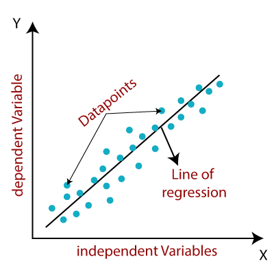
The linear regression model provides a sloped straight line representing the relationship between the variables. Consider the below image:

Mathematically, we can represent a linear regression as:

y= a₀+a₁x+ ε

Here,

Y= Dependent Variable (Target Variable)
X= Independent Variable (predictor Variable)
a0= intercept of the line (Gives an additional degree of freedom)
a1 = Linear regression coefficient (scale factor to each input value).
ε = random error

The values for x and y variables are training datasets for Linear Regression model representation.

Types of Linear Regression

Linear regression can be further divided into two types of the algorithm:

Simple Linear Regression:
If a single independent variable is used to predict the value of a numerical dependent variable, then such a Linear Regression algorithm is called Simple Linear Regression.
Multiple Linear regression:
If more than one independent variable is used to predict the value of a numerical dependent variable, then such a Linear Regression algorithm is called Multiple Linear Regression.

Linear Regression Line

A linear line showing the relationship between the dependent and independent variables is called a regression line. A regression line can show two types of relationship:

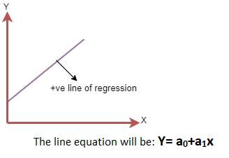
Positive Linear Relationship:
If the dependent variable increases on the Y-axis and independent variable increases on X-axis, then such a relationship is termed as a Positive linear relationship.

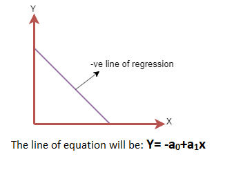
Negative Linear Relationship:
If the dependent variable decreases on the Y-axis and independent variable increases on the X-axis, then such a relationship is called a negative linear relationship.

Finding the best fit line:

When working with linear regression, our main goal is to find the best fit line that means the error between predicted values and actual values should be minimized. The best fit line will have the least error.

The different values for weights or the coefficient of lines (a₀, a₁) gives a different line of regression, so we need to calculate the best values for a₀ and a₁ to find the best fit line, so to calculate this we use cost function.

Cost function-

The different values for weights or coefficient of lines (a₀, a₁) gives the different line of regression, and the cost function is used to estimate the values of the coefficient for the best fit line.
Cost function optimizes the regression coefficients or weights. It measures how a linear regression model is performing.
We can use the cost function to find the accuracy of the mapping function, which maps the input variable to the output variable. This mapping function is also known as Hypothesis function.

For Linear Regression, we use the Mean Squared Error (MSE) cost function, which is the average of squared error occurred between the predicted values and actual values. It can be written as:

For the above linear equation, MSE can be calculated as:

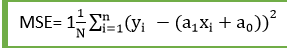
Where,

N=Total number of observation
Yi = Actual value
(a1x_i+a₀)= Predicted value.

Residuals: The distance between the actual value and predicted values is called residual. If the observed points are far from the regression line, then the residual will be high, and so cost function will high. If the scatter points are close to the regression line, then the residual will be small and hence the cost function.

Gradient Descent:

Gradient descent is used to minimize the MSE by calculating the gradient of the cost function.
A regression model uses gradient descent to update the coefficients of the line by reducing the cost function.
It is done by a random selection of values of coefficient and then iteratively update the values to reach the minimum cost function.

Model Performance:

The Goodness of fit determines how the line of regression fits the set of observations. The process of finding the best model out of various models is called optimization. It can be achieved by below method:

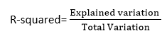
1. R-squared method:

R-squared is a statistical method that determines the goodness of fit.
It measures the strength of the relationship between the dependent and independent variables on a scale of 0-100%.
The high value of R-square determines the less difference between the predicted values and actual values and hence represents a good model.
It is also called a coefficient of determination, or coefficient of multiple determination for multiple regression.
It can be calculated from the below formula:

Assumptions of Linear Regression

Below are some important assumptions of Linear Regression. These are some formal checks while building a Linear Regression model, which ensures to get the best possible result from the given dataset.

Linear relationship between the features and target:
Linear regression assumes the linear relationship between the dependent and independent variables.
Small or no multicollinearity between the features:
Multicollinearity means high-correlation between the independent variables. Due to multicollinearity, it may difficult to find the true relationship between the predictors and target variables. Or we can say, it is difficult to determine which predictor variable is affecting the target variable and which is not. So, the model assumes either little or no multicollinearity between the features or independent variables.
Homoscedasticity Assumption:
Homoscedasticity is a situation when the error term is the same for all the values of independent variables. With homoscedasticity, there should be no clear pattern distribution of data in the scatter plot.
Normal distribution of error terms:
Linear regression assumes that the error term should follow the normal distribution pattern. If error terms are not normally distributed, then confidence intervals will become either too wide or too narrow, which may cause difficulties in finding coefficients.
It can be checked using the q-q plot. If the plot shows a straight line without any deviation, which means the error is normally distributed.
No autocorrelations:
The linear regression model assumes no autocorrelation in error terms. If there will be any correlation in the error term, then it will drastically reduce the accuracy of the model. Autocorrelation usually occurs if there is a dependency between residual errors.