Simple Linear Regression in Machine Learning

Simple Linear Regression is a type of Regression algorithms that models the relationship between a dependent variable and a single independent variable. The relationship shown by a Simple Linear Regression model is linear or a sloped straight line, hence it is called Simple Linear Regression.

The key point in Simple Linear Regression is that the dependent variable must be a continuous/real value. However, the independent variable can be measured on continuous or categorical values.

Simple Linear regression algorithm has mainly two objectives:

• Model the relationship between the two variables. Such as the relationship between Income and expenditure, experience and Salary, etc.
• Forecasting new observations. Such as Weather forecasting according to temperature, Revenue of a company according to the investments in a year, etc.

Simple Linear Regression Model:

The Simple Linear Regression model can be represented using the below equation:

y= a0+a1x+ ε 

Where,

a0= It is the intercept of the Regression line (can be obtained putting x=0)
a1= It is the slope of the regression line, which tells whether the line is increasing or decreasing.
ε = The error term. (For a good model it will be negligible)

Implementation of Simple Linear Regression Algorithm using Python

Problem Statement example for Simple Linear Regression:

Here we are taking a dataset that has two variables: salary (dependent variable) and experience (Independent variable). The goals of this problem is:

• We want to find out if there is any correlation between these two variables
• We will find the best fit line for the dataset.
• How the dependent variable is changing by changing the independent variable.

In this section, we will create a Simple Linear Regression model to find out the best fitting line for representing the relationship between these two variables.

To implement the Simple Linear regression model in machine learning using Python, we need to follow the below steps:

Step-1: Data Pre-processing

The first step for creating the Simple Linear Regression model is data pre-processing. We have already done it earlier in this tutorial. But there will be some changes, which are given in the below steps:

• First, we will import the three important libraries, which will help us for loading the dataset, plotting the graphs, and creating the Simple Linear Regression model.

• Next, we will load the dataset into our code:

By executing the above line of code (ctrl+ENTER), we can read the dataset on our Spyder IDE screen by clicking on the variable explorer option.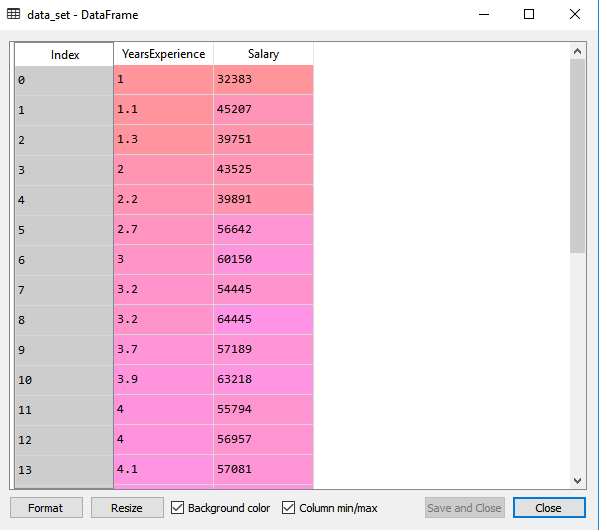

The above output shows the dataset, which has two variables: Salary and Experience.

Note: In Spyder IDE, the folder containing the code file must be saved as a working directory, and the dataset or csv file should be in the same folder.

• After that, we need to extract the dependent and independent variables from the given dataset. The independent variable is years of experience, and the dependent variable is salary. Below is code for it:

In the above lines of code, for x variable, we have taken -1 value since we want to remove the last column from the dataset. For y variable, we have taken 1 value as a parameter, since we want to extract the second column and indexing starts from the zero.

By executing the above line of code, we will get the output for X and Y variable as: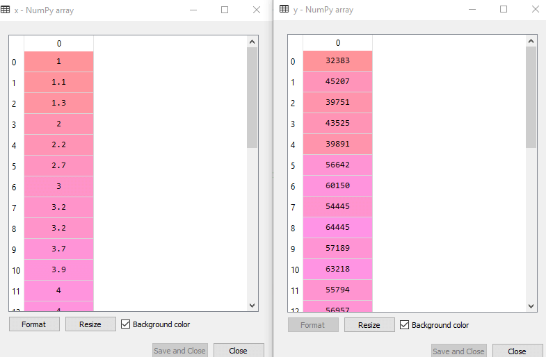

In the above output image, we can see the X (independent) variable and Y (dependent) variable has been extracted from the given dataset.

• Next, we will split both variables into the test set and training set. We have 30 observations, so we will take 20 observations for the training set and 10 observations for the test set. We are splitting our dataset so that we can train our model using a training dataset and then test the model using a test dataset. The code for this is given below:

By executing the above code, we will get x-test, x-train and y-test, y-train dataset. Consider the below images:

Test-dataset: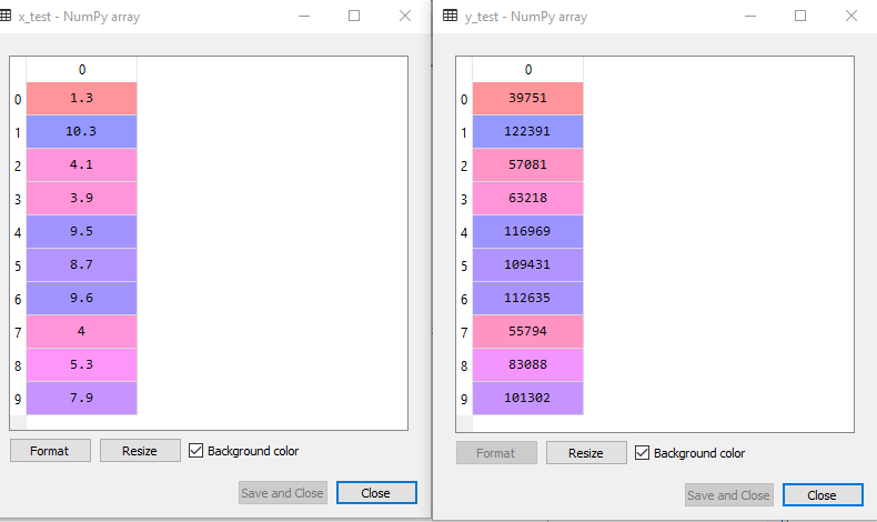

Training Dataset: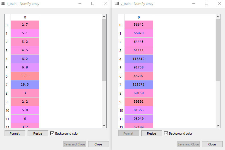

• For simple linear Regression, we will not use Feature Scaling. Because Python libraries take care of it for some cases, so we don't need to perform it here. Now, our dataset is well prepared to work on it and we are going to start building a Simple Linear Regression model for the given problem.

Step-2: Fitting the Simple Linear Regression to the Training Set:

Now the second step is to fit our model to the training dataset. To do so, we will import the LinearRegression class of the linear_model library from the scikit learn. After importing the class, we are going to create an object of the class named as a regressor. The code for this is given below:

In the above code, we have used a fit() method to fit our Simple Linear Regression object to the training set. In the fit() function, we have passed the x_train and y_train, which is our training dataset for the dependent and an independent variable. We have fitted our regressor object to the training set so that the model can easily learn the correlations between the predictor and target variables. After executing the above lines of code, we will get the below output.

Output:

Out[7]: LinearRegression(copy_X=True, fit_intercept=True, n_jobs=None, normalize=False)

Step: 3. Prediction of test set result:

dependent (salary) and an independent variable (Experience). So, now, our model is ready to predict the output for the new observations. In this step, we will provide the test dataset (new observations) to the model to check whether it can predict the correct output or not.

We will create a prediction vector y_pred, and x_pred, which will contain predictions of test dataset, and prediction of training set respectively.

On executing the above lines of code, two variables named y_pred and x_pred will generate in the variable explorer options that contain salary predictions for the training set and test set.

Output:

You can check the variable by clicking on the variable explorer option in the IDE, and also compare the result by comparing values from y_pred and y_test. By comparing these values, we can check how good our model is performing.

Step: 4. visualizing the Training set results:

Now in this step, we will visualize the training set result. To do so, we will use the scatter() function of the pyplot library, which we have already imported in the pre-processing step. The scatter () function will create a scatter plot of observations.

In the x-axis, we will plot the Years of Experience of employees and on the y-axis, salary of employees. In the function, we will pass the real values of training set, which means a year of experience x_train, training set of Salaries y_train, and color of the observations. Here we are taking a green color for the observation, but it can be any color as per the choice.

Now, we need to plot the regression line, so for this, we will use the plot() function of the pyplot library. In this function, we will pass the years of experience for training set, predicted salary for training set x_pred, and color of the line.

Next, we will give the title for the plot. So here, we will use the title() function of the pyplot library and pass the name ("Salary vs Experience (Training Dataset)".

After that, we will assign labels for x-axis and y-axis using xlabel() and ylabel() function.

Finally, we will represent all above things in a graph using show(). The code is given below:

Output:

By executing the above lines of code, we will get the below graph plot as an output.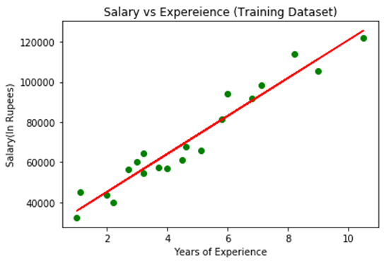

In the above plot, we can see the real values observations in green dots and predicted values are covered by the red regression line. The regression line shows a correlation between the dependent and independent variable.

The good fit of the line can be observed by calculating the difference between actual values and predicted values. But as we can see in the above plot, most of the observations are close to the regression line, hence our model is good for the training set.

Step: 5. visualizing the Test set results:

In the previous step, we have visualized the performance of our model on the training set. Now, we will do the same for the Test set. The complete code will remain the same as the above code, except in this, we will use x_test, and y_test instead of x_train and y_train.

Here we are also changing the color of observations and regression line to differentiate between the two plots, but it is optional.

Output:

By executing the above line of code, we will get the output as: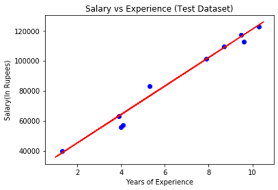

In the above plot, there are observations given by the blue color, and prediction is given by the red regression line. As we can see, most of the observations are close to the regression line, hence we can say our Simple Linear Regression is a good model and able to make good predictions.