Linear regression

Linear regression is a statistical method for modelling the connection among a scalar output and one or more causal factors (also called independent and dependent variables). The regression equation is used when there is only one independent factor; regression analysis is used when there is more than one independent factor. This phrase differs from multidimensional linear regression, which predicts several linked dependent variables instead of a single scalar variable.

Connections are represented using linear predictor equations whose uncertain parameter values are derived from information in linear regression. These kinds of models are known as linear models. The conditioned average of the answer based on the values of the independent variable (or predictors) is most typically believed to be a linear combination of those numbers. Linear regression, like other kinds of regression analysis, concentrates on the conditional distribution of the answer to providing the attribute values instead of the joint distribution of all of these factors, which is the realm of the multivariate model.

Linear regression was the first form of logistic regression to be carefully explored and widely employed in real-world applications. It is due to the fact that equations that are linearly connected to their uncertain variables are able to arrange than systems that are non-linearly connected to their factors, and the statistical methods of the generated estimation techniques are easier to recognize.

Linear regression offers a wide range of applications. The majority of applications fall into two main groups:

If predicting forecast, or reduced errors are the goals; linear regression can be used to adapt a statistical model to an acquired given dataset of responder and exogenous variables data. If new values of the independent variable are obtained without an associated expected value after creating a rather structure, the controller module may be used to assess the effects.
If the purpose is to examine differences in the dependent variables due to change in the causal variables, linear regression analysis may be used to assess the strength of the relationships among the reaction and the informative factors. Evaluate if any explanatory factors have no linear link with the answer at all, or find whichever subgroups of independent variables include redundant data about the answer.

Linear regression techniques are commonly equipped using the ordinary least square method, but they can also be designed to fit in other manners, including by reducing the "discrepancy" in another standard (as in median squares divergences regression) or by limiting a punished edition of the loss function objective functions (as in ridge regression (L²-norm penalty) and lasso regression) (L¹-norm penalty).

On the other hand, the least-square technique may be used to fit models that are not quadratic. As a result, via the phrases "linear model" and "least squares" are sometimes used interchangeably, they are not equivalent.

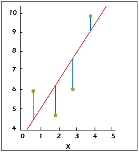
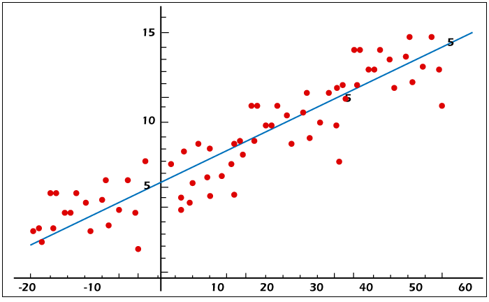
The data (red) in linear regression are supposed to be the consequence of arbitrary variations (green) from an inherent connection (blue) among a predictor variable (y) and an independent variable (x).

Introduction

A linear regression model with an input collection {yi, xi ,..., xip}i=1ⁿ of n statistical units implies that the correlation between the explanatory variable y and the p-vector of regression analysis x is constant. This link is represented by error terms or error variable ε, which is an uncontrolled probability distribution that introduces "noise" to the linear connection among the regressors and dependent variable. As a result, the model has the following equation:

yi = β₀ + β_1xi1 + ... + β_pxip + ε = x^Ti β + εi, i = 1,...,n,

T signifies the inversion in this case, therefore xiT β is the internal stresses of feature vector xi and β.

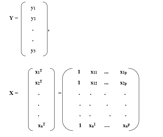
These n solutions are frequently layered together and represented in mathematical terms as-

Y = Xβ + ε,

Here,

Some words on sign and nomenclature:

Y is a matrix of observable values of the variable known as the regress and exogenous variables, dependent variables, measured variable, independent variables, or predictor variables, y_i= i=1,...,n. This variable is also referred to as the predicted variable. However, it should not be conflated with expected results, which are indicated by the symbol y^.
X can be represented as a vector of line-vectors xi or n-dimensional column-vectors xj, which are referred to as regression analysis, explanatory variable, independent variable, confounders, input data, dependent variable, or outcome variable. The design matrix is another name for vector X.

A steady is usually added as one of the regression coefficients. Specifically, xi0=1 for i=1,...,n. The comparable variable is referred to as the interceptor. Several appropriate statistical processes for linear models necessitate the presence of an intercept. Therefore it is frequently maintained even when different theories imply that it should be zero.
As in polynomial and segmented extrapolation, one of the regression coefficients might be a non-linear combination of some other regressor or of the information. The model is particularly linear as far as the parameter vector is straight.
The values xij might be interpreted as either observed data of response variable Xj or as a constant value determined before monitoring the dependent variable.
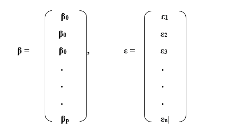
β is a (p+1)-dimensional parameter vector, with β0 representing the slope factor (if one is included in the equation; alternatively, β is p-dimensional). Its constituents are referred to as consequences or correlation coefficients. This parametric vector member is understood as the differential equation of the explanatory variable with regard to the numerous independent variables.
ε is a variable of εi ideal. This component is known as the standard error, perturbation phrase, or acoustic period (in contrast with the "signal" offered by the rest of the prototype). It includes all considerations other than the regressors x that explain the dependent variable y. The correlation among the error term and the regressors, such as their similarity, is critical in developing a linear regression prototype because it determines the effective analysis strategy.

Example

Assume a circumstance where a small sphere is being flung up in the air, and then we evaluate its altitudes of ascension hi at various times in time ti. Physics informs us that, neglecting the friction, the connection may be described as follows-

h_i = β₁t_i + β₂t_i² + εi,

Here, 1 is the sphere's starting motion, 2 is equivalent to standard gravity, and I is attributable to observation mistakes. Linear regression may be used to predict 1 and 2 variables from observed information. This paradigm is non-linear in duration but linear in variables 1 and 2; if we pick regressors xi = (x_i1, x_i2) = (t_i, t_i2), the approach takes on the conventional form-

h_i = x_i^T β + εi

Assertions

Conventional linear regression models, when used with conventional estimate procedures, generate a series of assertions about the response variables, predictor variables, and their relation. There have been several modifications that enable each of these premises to be loosened (i.e., decreased to a weaker version), and in some circumstances, abolished completely. In practice, these additions complicate and lengthen the estimating technique and may necessitate additional information in a way to construct an adequately exact model.

The primary arguments presented by typical linear regression models using conventional estimating techniques are as follows:

Exogeneity is lacking
This indicates that the predictive variables x can be viewed as a constant value instead of explanatory variables. It implies that the independent variable is believed to be error-free-that is, devoid of evaluation mistakes. However, this premise is unrealistic across many situations; abandoning it results in substantially more complicated errors-in-variables systems.
Linearity
This suggests that the responder variable's average is a linear mixture of the characteristics (regression coefficients) and dependent variable. It's worth noting that this premise is far less restricted than it appears. Since the regression models are viewed as a constant value (as discussed before), linearity is only a parametric constraint. The predictive variables individually can be freely altered, and many versions of the similar underlying predictor variable, each modified slightly, can be appended. This approach is used in polynomial regression, which employs linear regression to estimate the dependent variables as an unbounded transfer equation of independent variables (up to a specified order). Equations with this much adaptability, including such polynomial regression, frequently have "excessively capacity," in that they heavily influence the information. As a consequence, some form of normalization is usually required to avoid implausible answers from emerging from the estimating process. Ridge regression and logistic regression are common manifestations. Bayesian linear regression, which is almost resistant to the issue of computational complexity, can also be used. (In truth, lasso regression and ridge regression are both subsets of Bayesian linear regression, with different types of probability distribution used to the regression equation).
Constant variance
This suggests that the variability of the mistakes is independent of the predictor variables' quantities. Hence, irrespective of how great or little the answers are, the variance of the replies for specified constant value of the predictions is the similar. This is not always the case, because a statistic with a high mean has a higher variance than one with a low average. For instance, an individual whose revenue is forecasted to be $100,000 may conveniently have an investment return of $80,000 or $120,000-i.e., a margin of error of around $20,000-whereas a participant whose revenue is anticipated to be $10,000 is doubtful to have the similar $20,000 confidence interval, because their earned amount could range approximately $10,000 and $30,000. Heteroscedasticity is the lack of homoscedasticity. To test this premise, evaluate a chart of royalties' vs predicted values (or the results within each recently identified) for a "fanning impact."
A graph of the actual or cubed royalty's vs the anticipated numbers (or each classifier) can be used to look for trends or curvature. Formal tests can also be performed. When heteroscedasticity exists, a general "mean" assessment of variation is used rather than one that takes into consideration the underlying variation pattern. This results in less exact (but not skewed) estimated coefficients and prejudiced error variance, leading in deceptive tests and range values (in the instance of ordinary least squares). The model's standard error will also be incorrect.
Error Independence
This implies that the response variable mistakes are unrelated to one another. (Real statistical independence is a stronger requirement than simply the absence of correlation and is generally unnecessary, but it can be used if it is called to exist.) Certain approaches, including such modified linear regression, can handle associated errors, but they usually require substantially more information unless some kind of normalization is applied to tilt the system towards presuming uncorrelated mistakes. A basic approach to this problem is Bayesian linear regression.
The predictors do not have complete multicollinearity
The design matrix X must have a complete unit value p for traditional linear regression analytical techniques. Alternatively, complete multicollinearity occurs in the regression model, indicating a linear connection among two or more predictor variables. This can occur as a result of inadvertently modifying a factor in the information, using a linear transformation of a factor back to the original (for example, the similar temperature measurements demonstrated in Celsius and Fahrenheit), or such as a linear integration of various variables in the model, including their average value. It can also occur if there is insufficient data provided in comparison to the number of variables to be evaluated (e.g., fewer information spots than regression factors). Near breaches of this rule, when predictors are substantially but not fully linked, might impair parameter estimation accuracy.
The parameter vector β will be anti-identifiable in the event of complete multicollinearity-it has no specific value. Only a subset of the characteristics can be recognized in this scenario. In other words, their estimates can only be approximated inside a linear subdomain of the whole real number R_p.

Methodologies for suitable multicollinear linear models were generated, some of which require extra presumptions, including such "effect sparsity" that a significant portion of the consequences is precisely zero. It is worth noting that more computationally complex elaborated prediction algorithms, like those used in generalized linear models, are not affected by this issue.

Aside from these hypotheses, numerous other statistical features of the information have a significant impact on the efficacy of various estimate methodologies:

The statistical link among the error terms and the regressors are critical in assessing if an estimating technique has acceptable selection qualities like unbiasedness and consistency.
The ordering, or conditional probabilities, of the response variable x has a significant impact on the accuracy of estimations of β. Sampling and inferential statistics are well-established subcategories of statistics that give guidelines for gathering information in such a manner that an accurate prediction may be obtained.

Projection

When all of the previous predictive variables in the study are "kept constant," a built linear regression framework can be used to find the connection among a particular response variable y and predictor variable xj. The meaning of βj is the anticipated shift in y for each shift in xj if the other variables are held constant that is the net present value is estimated parameters with regard to xj. It is commonly referred to as xj's one-of-a-kind influence on y. The negligible impact of xj on y, on the other hand, may be determined using a linear relationship or a basic linear regression model that simply relates xj to y; this impact is the entire gradient of function with respect to xj.

When analyzing regression findings, keep in mind that certain regressors (like sample variables or the slope factor) may not permit for small alterations, while others cannot be maintained constant (revoke the instance from the introduction: it would be not possible to "retain t_i fixed" and at the similar period alter the value of ti²).

Even though the negligible impact is substantial, the distinct impact may be almost nil. It means that another factorial contains all of the data in xj, such as once that factor is included in the equation, xj no longer contributes to the variance in y. In contrast, xj's distinctive impact might be significant while its negligible impact is essentially insignificant. This would occur if the other factors accounted for a significant portion of the variance in y, but only in a complementary manner to what xj captures. In this scenario, incorporating the other parameters into the model minimizes the portion of y's variation that is related to xj, so enhancing the integrative manner with xj.

Enhancements

Many linear regression modifications have been created, allowing some or all of the assertions underlying the general structure to be loosened.

Simple and multiple linear regression

Simple linear regression is the most basic instance of a numerical value explanatory variables x and a real-valued responder parameter y. Many linear regression, also called multidimensional linear regression, is the expansion to multiple and/or quaternion predictor variables (signified with a letter X).

Multiple linear regression is an extension of basic linear regression with more than one exponential function and a subset of universal linear regression with just one predictor variables. The underlying assets for many linear regression is as follows:

Y_i = β₀ + β_1xi1 + β_2xi2 + ... + β_pxip + εi

i = 1,..., n for each discovery

We assume n occurrences of one predictor variable and p exogenous variables in the calculation. As a result, Y_i is the ith assumption of the predictor variables, and X_ij is the i^th analysis of the j^th exponential function, with j = 1, 2,..., p. The numbers βj reflects the estimation technique, while εi represents the i^th independent identically distributed standard deviation.

In the more extensive multimodal linear regression, one expression of the following form is used for each of m > 1 control variables that contain a similar set of exogenous factors and are therefore evaluated concurrently.

Y_i = β_0j + β_1jX_i1 + β_2jX_i2 + ... + β_pjX_ip + εij

Including all observations denoted by I = 1,..., n and all response variables denoted by j = 1,..., m.

Almost all legitimate regression models include many variables, and fundamental presentations of linear regression are frequently written in the context of the various regression model. Therefore, in these circumstances, the dependent variables y remains a vector.

General linear model

The generic linear model takes into account the case where the responder variable, yi, is a matrix rather than an integer (for each measurement). The equation E = (y|xi) = xi^TB intrinsic normality is still maintained, with a vector B substituting the matrix of the traditional linear regression model. There have been created multidimensional equivalents of conventional least squares (CLS) and generalized least squares (GLS). "Multivariate linear models" are another name for "generic linear models." These are not to be confused with multivariate linear regression (also identified as "multiple linear models").

Models with heteroscedasticity

Several methods have been proposed to account for heteroscedasticity, which means that the variations of faults for distinct response variables may fluctuate. Loaded least-square, for instance, is a technique for assessing linear regression models where the answer factors have various error values, sometimes with linked failures. Heteroscedasticity-consistent standard deviation is a more accurate technique for dealing with non-overlapping but perhaps heteroscedastic mistakes.

Generalized linear models (GLM)

Generalized linear models are a methodology for describing response variables that are either limited or continuous. This is used in situations such as:

When sculpting favorable amounts that differ on a massive scale are best explained by a statistical distribution including the log-normal allocation or Probability distribution (even though GLMs are not used for log-normal information, rather the dependent variable is merely converted using the logarithm purpose).
When descriptive simulation statistics, including the selection of a particular applicant in voting (which is best understood using a Bernoulli allocation spread for binary selections or a normative distribution/multinomial allocation for multi-way decisions), where there are a corrected variety of opportunities that cannot be substantively requested.
For representing descriptive statistics, such as evaluations on a scale of 0 to 5, where the results can be arranged, but the amount itself may not have any ultimate significance.
Generalized existing methods provide an optional linear model, g, which connects the average of the responder variable(s) to the indicators: E(Y)=g-1 (XB). The connection variable is frequently connected to the increasing effort, and it usually has the impact of converting among the (-?,?) region of the linear classifier and the domain of the dependent variables.

GLMs are commonly used in the following contexts:

For summary statistics, Poisson regression is used.
For binary information, logistic regression and probit regression are used.
For categorical information, multinomial probit regression and multinomial logistic regression are used.
For ordinal information, ordered probit regression and ordered logit are used.

Single index features require some deformations in the connection among x and y while maintaining the significant role of the linear predictor β?x as in the conventional linear regression model. Actually, returning OLS to information from a single system will equivalent resistance β up to a proportional factor under specific situations.

Linear models with hierarchies

Hierarchical linear models (or multilayer imputation) arrange information into a pyramid of regressions, such as A being based on B, and B being reported on C. It is often used in academic analytics, where children are buried in classes, classes are contained in institutions, and institutions are contained in an administrative unit, including an education department.

Errors-in-variables

Errors-in-variables approaches (also known as "measurement error methods") expand the basic linear regression model by allowing explanatory variables X to be measured with inaccuracy. Conventional approximations become skewed as a result of this mistake. The most common type of bias is absorption, which means that the impacts are skewed around zero.

Some other approaches

Linear regression analysis in Dempster-Shafer concept, or a linear faith value specifically, may be expressed as a partly swept vector that may be coupled with equivalent vectors expressing observations and other specified probability distribution and phase formulas. Combining swept and unswept matrices offers an additional technique for generating linear regression models.

Approximation methods of Linear regression

A vast variety of techniques for estimation methods and interpretation in linear regression have been established. The supercomputing brevity of the methodologies, the existence of a closed-form remedy, the rigidity with reference to massive allocations, and the underlying concepts required to validate attractive statistical characteristics like accuracy and exponential reliability distinguish these techniques.

To demonstrate that the β produced is the feature vector, divide once more to produce the Hessian matrix and demonstrate that it is globally stable. The Gauss-Markov theorem provides this.

Linear least-squares techniques primarily include:

Least squares in practice
Least squares with weights
Least squares modified

Maximum-likelihood estimation and other related methods

When the dispersion of the constant variance is recognized to correspond to a specific functional group ?? of weibull distribution, a maximum likelihood assessment may be conducted. The resultant approximation ?? is equal to the OLS value where f is a simple model with zero mean and variance ?. Ridge regression or other kinds of biased calculation, including such Lasso regression, intentionally incorporate skew into the assessment in order to limit the estimate's variance. When ε reflects a symmetric distribution with a determined covariance matrix, GLS predictions are expectation-maximization estimates.
Ridge regression and other kinds of biased measurement, including such Lasso regression, intentionally incorporate error into the assessment of β in effort to reduce the estimate's volatility. The resultant estimations have reduced squared error than OLS approximations, especially when multi-collinearity is prevalent or generalization is an issue. They are often employed when the aim is to forecast the amount of the dependent variables y given unobserved quantities of the predictors x.
Least absolute deviation (LAD) modelling is a more stable estimate approach than OLS because it is less susceptible to extremes (but is less capable than OLS when no deviation is present). Maximum likelihood estimates for ε a Laplace dispersion model is similar.

Other methods of assessment

The concept of Bayesian statistics is applied to regression analysis in Bayesian linear regression. The confidence intervals are considered to be randomly initialized with a certain probability distribution. In a manner comparable to (but broad than) lasso regression or ridge regression, the covariance matrix might influence the values for the regression equation. Furthermore, the Bayesian estimation method generates a whole posterior distribution, which entirely describes the uncertainty regarding the item, rather than a single point approximation for the "best" outcomes of the correlation coefficient. This may be used to calculate the "best" parameters from the posterior distribution using the average, middle, maximum, any quantile, or any other metric.
Quantile regression, as opposed to conditional mean regression, concentrates on the contingent distributions of y given X. Linear quantile regression analyzes a specific contingent absolute value, such as the implicit median, as a normal distribution of the predictors βTx.
When the connections have a defined structure, hybrid models are commonly employed to evaluate linear regression connections, including response variables. Hybrid models are commonly used to analyze the information requiring multiple measures, including such longitudinal data or data collected by sampling frame. They are often fitted as stochastic methods with either maximum likelihood or Bayesian approximation. There is a tight relationship among variables involved and multiple regression squares when the mistakes are treated as ordinary random variables. Panel data estimate is another method for evaluating this sort of information.
When the amount of independent variable is big, or there are significant correlations between the response variable, principal component regression (PCR) is used. The independent variable is minimized utilizing principal component analysis in the initial step, and then the decreased variables are used in an OLS regression model in the second phase. While it frequently performs well in reality, there is no theoretical frameworks reason why the most relevant linear function of the independent variable should be between the dominating key elements of the predictive variables' multimodal distribution. The fractional least squares regression model is an adaptation of the PCR method that does not have the aforementioned flaw.
Least-angle regression is a linear regression model estimate technique designed to manage high-dimensional correlated matrices, perhaps with more confounders than events.
Theil-Sen estimator is a straightforward resilient estimating approach that selects the gradient of the fitted model as the midpoint of the gradients of the lines passing between sets of line segments. It has empirical performance features comparable to basic linear regression but is significantly more robust to small.
Several robust estimate approaches have been proposed, such as the ?-trimmed mean approaches and L-, M-, S-, and R-estimators.

Application area of Linear regression

Linear regression is frequently used to determine probable connections among variables in biological, social sciences and behavioral. It is regarded as the essential instrument in these fields.