| |

Kohonen Self-Organizing MapsThe self-organizing maps were invented in the 1980s by Teuvo Kohonen, which are sometimes called the Kohonen maps. Since they have a special property that efficiently creates spatially organized "inner illustrations" for the input data's several features, thus it is utilized for reducing the dimensionality. The topological relationship amid the data points is optimally preserved by the mapping. Consider Figure 1. given below and try to understand the basic structure of the self-organizing map network. It has an array that constitutes neurons or cells, which are set out on a rectangular or hexagonal sheet. Here the cells are denoted as the single index i, such that the input vector X(t)= [ x1(t), x2(t), ..., xn(t)]T ∈ Rn is connected parallelly to all the cells, through different weight vectors mi(t) = [ mil(t), mi2(t) ..., min(t) ∈ Rn that are further adapted as per the input data set all through the self-organizing learning procedure. 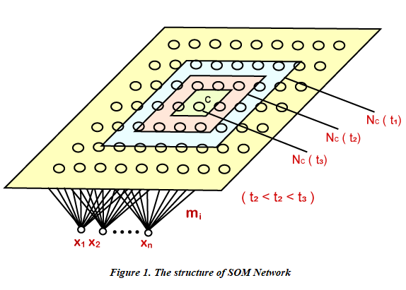
Firstly, we initialize the mi(0)'s with some small random values at the time of procedure learning, and then we repeatedly present the data, which has to be analyzed as an input vector either in the original order or some random order. Each time we present an input X(t), we come across the best-matching cell c among all the cells, which is defined as below; 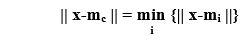
where ||. || represents the Euclidean distance or measurement of some other distance. We have defined a neighborhood Nc (t) around the cell as a range of lateral interaction, which has been demonstrated in the above figure. The basic weight-learning or weight adapting process is ruled by the following equation: 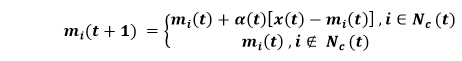
Here, 0 <α(f) < 1 relates to a scalar factor, which is responsible for controlling the learning rate that must decrease with time so as to get good performance. As a result of lateral interaction, the network tends out to be spatially "organized" after adequate self-learning steps as per the input data set's structure. The cells also get tuned to some particular input vectors or groups of them, where each cell is responsible for responding only to some specific patterns within the input pattern set. Lastly, the cell locations of those cells that respond to different inputs incline to be well-organized according to the topological relations amid the pattern inside the input set. In this way, it helps in optimal preserving of topological relationships in the original data space on the neural map, which is why it is known as Self-Organizing Map as it makes the network quite powerful in certain applications. Self-organizing Map AnalysisLet us assume if cell i acknowledges the input vector X; then we call cell i or its location on the map just like an image of the input vector X. Every pattern vector in the input set has only one image on the neural map, but one cell can be the image of many vectors. In the case, if a lattice is placed over a plane, and we incorporate it for representing a neural map, then, in that case, one square corresponds to one neuron followed by writing a number of the input pattern, whose image is represented by the cell existing in the corresponding square and we get a map as shown in Figure 2. The map portrays the distribution of the input patterns images over the neural map, which is why it is termed as SOM density map or SOM image distribution map. 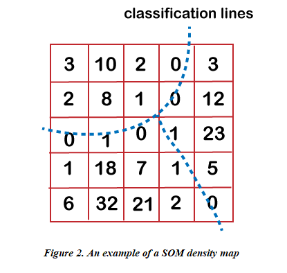
Every time there occurs groupings or clustering within the original pattern set, SOM will preserve it and showcase on the SOM density map, which is nothing, but the consequence of lateral competition. Closer patterns residing in the original space will "crowd" their images in some place on the map, and since the cells amid two or more image-crowded places are influenced by both the adjacent clusters, they will incline to respond to none of them. They will be imitated as some "plateaus" representing the clusters within the dataset that are separated by some "valleys", which corresponds to the classification lines on the SOM density map. Consider Figure 2 to have a better understanding of this phenomenon. The classification lines are drawn by dotted lines in the figure. This is the basis on which we do cluster analysis through the self-organizing map. We analyze the data for "training" the SOM, and then after undergoing "learning", the clusters are portrayed on the SOM density map. Following are some of its advantages:
Building a SOMWe are going to implement our first unsupervised deep learning model, i.e., Self-Organizing Maps, to solve a new kind of business problem, which is Fraud detection. So, in order to understand the business problem before starting with its implementation, let's suppose that we are a deep learning scientist working for a bank, and we are given a dataset that contains information of customers from this bank applying for an advanced credit card. Basically, this information is the data that customers had to provide when filling the application form. And our mission is to detect potential fraud within these applications, which means by the end of this mission, we have to give the explicit list of the customer who potentially cheated. So, our goal is very explicit. We have to return something, i.e., the list of potential fraudulent customers, we will not make a supervised deep learning model and try to predict if each customer potentially cheated or not with a dependent variable that has binary values. Instead, we will build an unsupervised deep learning model, which means we will identify some patterns in a high dimensional dataset full of nonlinear relationships, and one of them will be the potential frauds. We will start by importing the essential libraries in the same way as we did in our previous topics so that we can move on to implementing the model. Next, we will import the "Credit_Card_Applications.csv" dataset. We have taken our dataset from the UCI Machine Learning Repository, which is called Statlog Australian Credit Approval Dataset, and you can simply get by clicking on http://archive.ics.uci.edu/ml/datasets/statlog+(australian+credit+approval). After importing the dataset, we will go to the variable explorer and open it. 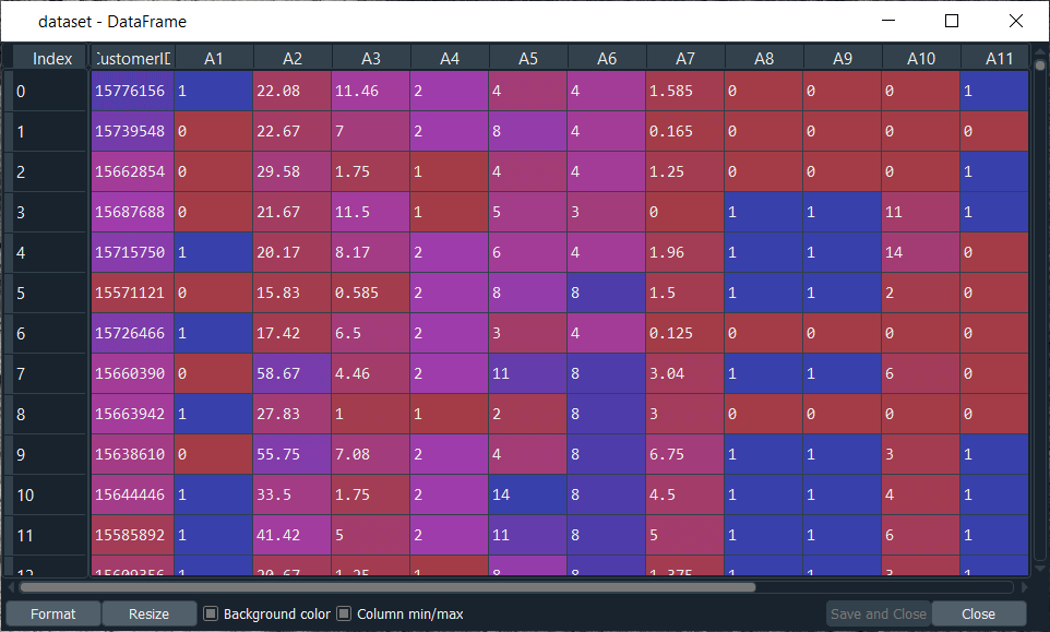
From the above image, the first thing we need to understand is that here the columns are the attributes, i.e., the information of the customers and the lines are the customers. Earlier, when we said that the unsupervised deep learning model is going to identify some patterns, which are the customers. These customers are the inputs of our neural network, which are going to be mapped to a new output space. In between the input space and the output space, we have a neural network composed of neurons, each neuron being initialized as a vector of weights that is the same as the vector of the customer, i.e., a vector of 15 elements, because we have the customer Id plus 14 attributes and so, for each observation point or each customer, the output of this customer will be the neuron, which is the closest to the customer. And this neuron is called the winning node for each customer, which is the most similar neuron to the customer. Next, we will use the neighborhood function like the Gaussian Neighbourhood function to update the weight of the neighbors of the winning node to move them closer to the point. We have to repeatedly do this for all the customers in the input space, and each time we repeat it, the output space decreases, followed by losing the dimensionality. It reduces the dimensions little by little. And then, it reaches a point where the neighborhood or output space stops decreasing, which is the moment where we obtain our self-organizing map in two-dimension with all the winning nodes that were eventually identified. It helps us in getting closer to the frauds because, indeed, when we think about frauds, we think about the outliers due to the fact that fraud is defined by something, which is far from general rules. The general rules are those rules, which must be respected when applying to the credit card. So, the frauds are actually the outlying neurons in the two-dimensional self-organizing maps because the outline neurons are far from the majority of neurons that follow the rules. Therefore, to detect the outline neurons in the SOM, we need the Mean Interneuron Distance, which means in our self-organizing map for each neuron, we are going to compute the mean of the Euclidean distance between one neuron and its neighborhood, such that we have to define the neighborhood manually. But we define a neighborhood for each neuron, and we compute the mean of the Euclidean distance between the neuron that we picked and all the neurons in the neighborhood, which we defined as if doing so we will be able to detect the outliers because outliers will be far from all the neurons in its neighborhood. After that, we will use an inverse mapping function to identify which customers originally in the input space are associated with the winning node, which is an outlier. So, here we have solved our mystery, we will start with its implementation part. We will first undergo the splitting of our dataset into two subsets, the sets that contain all the variables from customer ID to attribute number 14, i.e., A14, and the class, which is the variable that tells if Yes or No the application of the customer was approved. Therefore, 0 relates to No, the application was not approved, whereas 1 means Yes, the application was approved. Here we need to separate all these variables and the variable class, so that on the self-organizing map we can clearly distinguish between the customers who haven't approved their application and the customers who got approval because only then it will be useful as for example if we want to detect in priority, the fraudulent customers who got their applications approved that would actually make more sense. After importing the dataset, we will create those two subsets for which we will call a variable X, making it equal to dataset.iloc to get the indexes of the observations we want to include in X. So, we will start with indexed lines, and since we want all the lines because we want all the customers, we will use the : here and then as we want all the columns except the last one, we will use :-1. And then, as usual, we will use .values for the fact that it will return all the observations indexed by these indexes here. Next, we will create the last column, and for that, we will call it y. Since we are going to take the last column, so we only need to replace :-1 by -1, and the rest code remain the same as we did for the X variable. After executing the above two lines of code, X and Y will get created, which we can check on the variable explorer pane. From the image given below, we can clearly see that X contains all the variables except the last one. However, y contains the last variable that tells if Yes or No, the application was approved. Output: 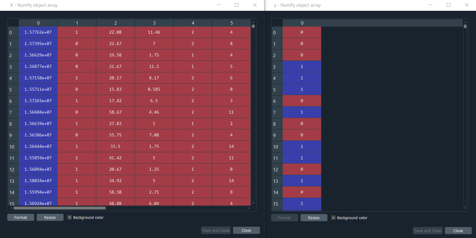
Note: Here we split our datasets into x and y, but we did not do that because we were doing some supervised learning, we are not trying to make a model that will predict 0 or 1 in the end. We are just going to make the distinction in the end between the customers who were approved and the customers who weren't approved.Since we are training our self-organizing map, we will only use X because we are doing some unsupervised deep learning, and with that, we mean no independent variable is being considered. Next, we will do feature scaling because it is compulsory for deep learning as there are high computations to make and we are going to start with a high dimensional dataset with lots of nonlinear relationships, so it will be much easier for our deep learning model to be trained if the features are scaled. We are actually going to do the same as we did for the Recurrent Neural Networks. We will use the normalization, which means we will get all our features between 0 and 1. So, we will start by importing the MinMaxScaler from sklearn.preprocessing. Then we will create an object sc of MinMaxScaler class, and inside the class, we will pass feature_range parameter that specifies the range of our scales in between 0 and 1, which is termed as normalization. Next, we will fit sc object to X so that sc gets all the information of X like the minimum and maximum, all the information that it needs to apply normalization to X. So, we will first fit the object to X, and then we will need to transform X, i.e., to apply normalization to X. Therefore, we will use the sc.fit_transform method that we will apply to X. After executing the above code, we can see from the below image that X is all normalized, we can indeed check all the values are between 0 and 1. Output: 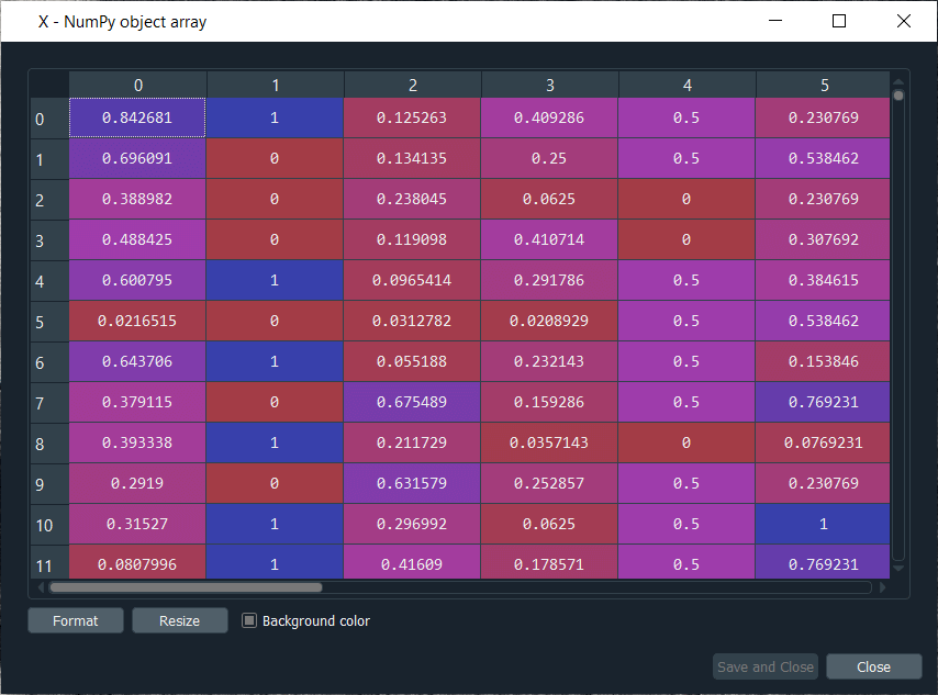
So, we just completed our data-pre-processing phase, and now we are ready to train our SOM model. To train our model, we have the following two options:
So, we will take it from another developer, which totally depends on what is available online and if some good implementations of SOM were made by developers. Fortunately, one such excellent implementation of SOM is Minisom 1.0, which is developed by Giuseppe Vettigili, and it is a NumPy based implementation of self-organizing maps. The license is Creative Commons by 3.0, which means we can share, adapt as well as do whatever we want to do with the code, so we can totally use it to build our SOM. To start with training the SOM model, we will first import the MiniSom keeping in mind that in our working directory folder in file explorer, we get the minisom.py, which is the implementation of the self-organizing map itself made by the developer. We will import the class called MiniSom from the minisom python file. Next, we will create an object of this class, which is going to be the self-organizing map itself that is going to be trained on X as we are doing some unsupervised learning, i.e., we are trained to identify some patterns inside the independent variables contained in X, and we don't use the information of the dependent variable. We don't consider the information in y. Since the object is the self-organizing map itself, so we will call it som, and then we will call the class MiniSom, and we will pass the following parameters inside it.
After this, we will train our som object on X, but before that, we will first initialize the weights, which we will do with the help of random_weights_init method and inside the method, we will input X. Then we will use the train_random method to train the som on X. Inside the method, we will pass two arguments; one is the data, i.e., X and the other is num_iteration, which is the number of iterations. Here we are trying with 100 iterations as it will be enough for our dataset. So, we have just trained our model, and now we are ready to visualize the results, i.e., to plot the self-organizing maps itself where we can clearly see the 2-dimensional grid that will contain all the final winning nodes, and for each of these winning nodes, we will get the Mean Interneuron Distance. The MID for each of a specific winning node is the mean of the distances of all the neurons around the winning node inside a neighborhood that we defined sigma, which is the radius of the neighborhood. So, higher the MID, more the winning node is an outlier, i.e., frauds because, for each neuron, we will get the MID for which we simply need to take the winning nodes that have the highest MID. In order to start building the map, we will need some specific functions to do this as we will not be using matplotlib because the plot that we are about to make is actually quite specific. We are not going to plot a classic graph like a histogram or curve, but we are building a self-organizing map, and therefore in some way, we are going to make it from scratch. So, the functions we will use, we will import from the pylab, and these functions are bone, pcolor, colorbar, plot, and show. Next, we will start making the map for which we will first need to initialize the figure, i.e., the window that will contain the map, and to do this, we will use the bone() function. In the next step, we will put the different wining nodes on the map, which we will do by adding the information of the Mean Interneuron Distance on the map for all the winning nodes that are identified by the SOM. Here we will not add the figures of all these MID instead we will use different colors corresponding to the different range values of the MID and to do this, we will use pcolor function inside of which we will add all the values of the MID for all the winning nodes of our SOM. In order to get these mean distances, we have some specific method, i.e., Distance Map method and in fact, this distance map method will return all the MID in one matrix followed by taking the transpose of the matrix to get the things in the right order for the pcolor function that will be done by using som.distance_map().T. Next, we will add the colorbar that will exactly give us legends of all these colors. 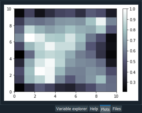
From the above image, we can see that we have the legends on the right side of the image, which is the range values of the MID. But these are the normalized values that were scaled from 0 to 1. therefore, we can clearly see the highest MID's correspond to the white color, and the smallest MID's corresponds to the dark color. So, based on what we discussed earlier, we already know where the frauds are because they are identified by the outlying winning nodes that are far from the general rules. It can be seen that all the majority of dark colors are close to each other because their MID is pretty low, which means all the winning nodes in the neighborhood of one winning node are close to the winning node at the center, which therefore creates the clusters of the winning node. Since the winning node has the large MID's, so they are outliers and accordingly potential frauds. In the next step, we will get the explicit list of customers by just proceeding to the inverse mapping of the winning node to see which customers are associated with that particular winning node. But we can do better than this map as we can add some markers to make the distinction between the customers who got approval and the customers who didn't get the approval because the customer who cheated and got approval are more relevant target to fraud detection than the customers who didn't get approval and cheated. Therefore, it would be good to see where the customers are in the self-organizing map. So, in the next step, we will add markers everywhere to tell for each of these winning nodes if the customer who is associated with these winning nodes got approval or not. We will create two markers; some red circles corresponding to the customers who didn't get approval and some green squares that relate to the customers who got approval. To create a marker, we will first create a new variable called markers, and then a vector of two elements corresponding to the two markers, i.e., the first one is the circle that is quoted by "o" and the other one is the square, which is quoted by "s". Next, we will color these markers for which we will again create a variable named as colors followed by creating a vector of two elements; the first one is the red color quoted by "r" and the green color quoted by "g". After this we will loop over all the customers and for each customer, we are going to get the winning node and depending on whether the customer got approval or not, we will color this winning node by the red circle if the customer didn't get the approval and a green square if the customer got approval. Here we will use a for loop that needs two looping variables, i.e., i and x, such that i is the different values of all the indexes of our customer database, which simply means it is going to take values from 0,1,2,..689 and x is going to be different vectors of the customer. So, for x and i, we will add in enumerate, and inside the enumerate, we will add X followed by entering into the loop. Inside the loop, we will first get the winning node for the first customer because, at the beginning of this loop, we start with the first customer for which to get its winning node. To get the winning node, we will start with w, and then we will take our object som, followed by taking the winner method. Next, we will pass X in the winner method as it will get us the winning node of the customer X. After getting the winning node, we will plot the colored marker on it. Then in plot function, we will specify the coordinates of the marker, and for that, we would like to place the marker at the center of the winning node. Since each winning node is represented by a square in the self-organizing map as we saw earlier, so we want to put the marker at the center of the square. Therefore the coordinates of the winning nodes are w[0] corresponds to X coordinates, and w[1] relates to y coordinates of the lower-left corner of the square. But we want to put at the center of the square, so we will add w[0] + 0.5 to put it in the middle of the horizontal base of the square and w[1] + 0.5 to put it at the center of the square. In order to know whether the marker is going to be a red circle or a green square, we will take the markers vector, which we created earlier and then we will pass y[i] inside the vector because i is the index of the customer, so y[i] is the value of the dependent variable for the customer, i.e., 0 if the customer didn't get the approval and 1 if the customer got the approval. Therefore, it can be concluded that if the customer didn't get the approval, then y[i] will be equal to 0, and so will be the markers[y[i]], i.e., a circle. Similarly, if the customer got approval, then y[i] and markers[y[i]] will become equal to 1, corresponding to a square. Next, we will add the colors in the same way, by taking our colors vector, i.e., colors and then we will take [y[i]] as it contains the information whether the customer got the approval of not, such that depending on the value of [y[i]], we will get a red, if the customer didn't get approval and green if the customer got approval. But in fact, we will give colors[y[i]] to the marker, however, in the markers, we can color the inside of the marker and the edge of the marker. Here we are going to color the edge of the marker, so we will make markeredgecolor equal to colors[y[i]], and for the inside of the marker, we will not color it because we can have two markers for the same winning node and therefore, we will make markerfacecolor equals to None. Lastly, we will add markersize because otherwise, we will get too small markers, and we want to be able to see the markers, so we will make it equal to 10. Eventually, we will do the same for the size of the edges; therefore, we will add markeredgewidth followed by setting it equal to 2. Now when we look at our self-organizing map, we will see it will actually look much better because not only we will see the differed Mean Interneuron Distances for all the winning node, but besides we will see the customer associated to the winning node are customers who got approval or not and to check it, we will add show() to show the graph. Output: 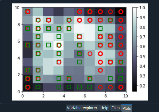
From the above image, we can see that we have the Mean Interneuron Distances as well as we get the information about whether the customers got approval or not for each of the winning nodes. For example, if we look at red circles, we can see that customers associated with that particular winning node didn't get the approval. However, if we look at green squares, we can see that the customers associating with it got the approval. Now, if we look at the outliers, then they are the winning nodes, where the Mean Interneuron Distances are almost equal to 1, indicating a high risk for the customers associating to those winning nodes. Basically, in that particular case, we see that we have both the cases, i.e., some customers got the approval, and some didn't get the approval because we get a green square as well as a red circle. So, now we have to catch the potential cheaters in the winning nodes but in priority those who got approval because it's of course much more relevant to the bank to catch the cheaters who got away with this. Here we are done with the map, it's quite good, and now we will use this map to catch these potential cheaters. We will use a dictionary, which we can obtain by using a method available in minisom.py as it contains all the different mappings from the winning nodes to the customer. Basically, we will first get all these mappings, and then we will use the coordinates of our outliers winning nodes that we identified, the white ones as it will give us the list of customers. Since we already identified two outlying winning nodes, well we will have to use the concatenate function to concatenate the two lists of customers, so that we can have a whole list of potential cheaters. We will start by introducing a snew variable mapping followed by using a method that will return the dictionary of all mappings from the winning nodes to the customers. Since it is a method, so we need to take our object som, and then we will add dot followed by adding the win_map method. Inside the method, we will simply input X, which is not the whole data, but only that data on which our SOM was trained. Upon execution of the above code, we will have the following output. Output: 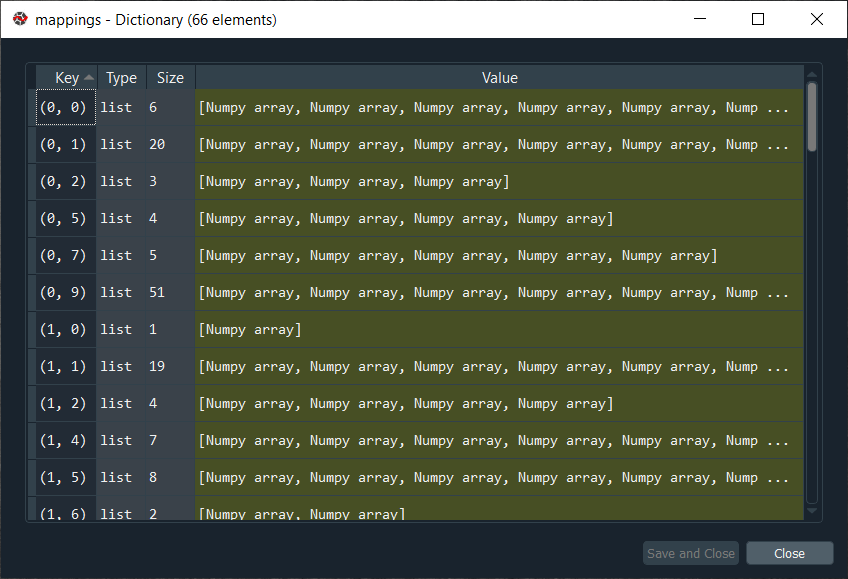
As we already said, mappings is actually a dictionary, and if we click on it, we will get all the mappings for all the different winning nodes in our SOM. Here the key is the coordinates of the winning nodes, and if we talk about the coordinates (0,0), we will see there are 6 customers associated with that particular winning node, and we can actually see the list by clicking on the corresponding value, which is shown as below. 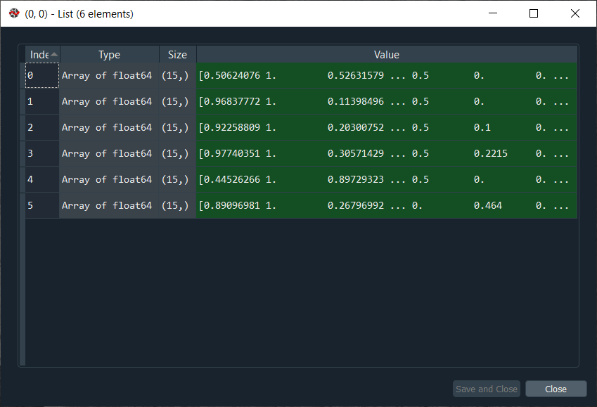
From the above image, each line corresponds to one customer that is associated with the winning node of coordinate (0,0). After this, we create a new variable called frauds, and then we will again go back to our map to get coordinated of the outlying winning node because these are the winning nodes that correspond to the customer, which we are looking for. So, we will execute it again, and then we will take the mappings dictionary. Inside the brackets of the dictionary, we will input the coordinates of the first outlying nodes, i.e. (1,1) as it will give us the list of the customers associated to this outlying winning node followed by adding the coordinates of second outlying winning nodes (4,1), which corresponds to very high MID. Here is one thing which is very important to keep in mind, i.e., whenever we input two lists that we are willing to concatenate into one same argument, we just need to put our two mappings into a new pair of parenthesis, and after that, we add the other argument, i.e., axis, which is a compulsory argument because that is how you specify if you want to concatenate vertically or horizontally. Since we are concatenating the horizontal vectors of customers as well as we want to put this second list of customer vectors below the first list of customer vectors, so we will concatenate along the vertical axis for which the default value is 0. Eventually, we are all set to get the whole list of cheaters, so let execute the following code. 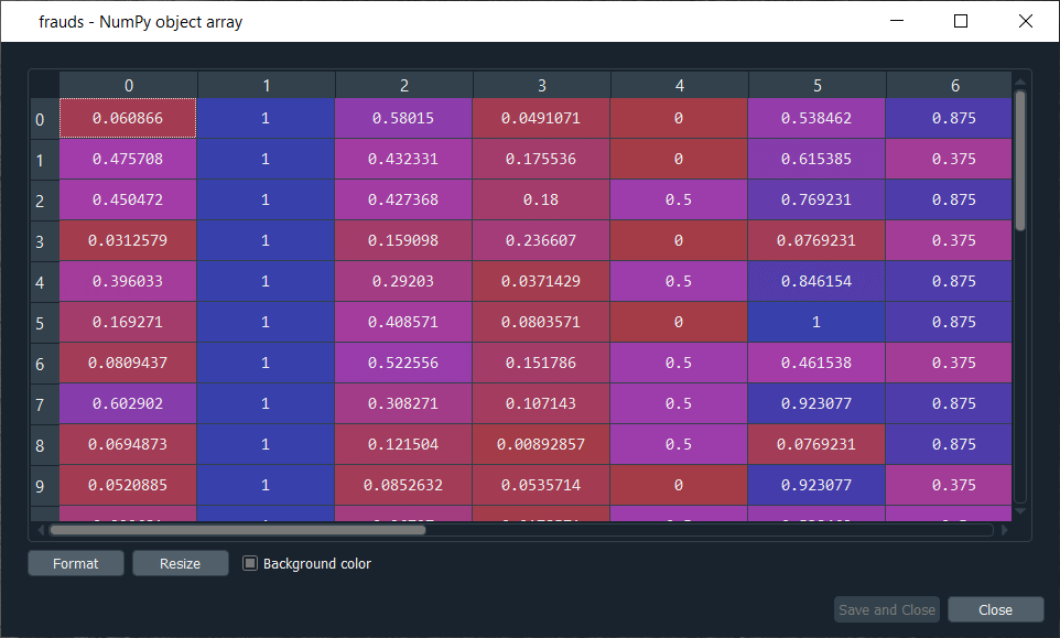
From the above image, we can see the list of customers who potentially cheated. We can see that the values are still scaled, so the only this left to do is to inverse the scaling, and to do that, we have an inverse scaling method that inverses this mapping. So, we will again start by taking the frauds list followed by using the inverse_transform method that will inverse this scaling. Since we applied the feature scaling with sc object that we created from the MinMaxScaler class, so we will take our object sc, and then we will use the inverse_transform method, and inside this method, we will enter the list of our frauds. When we run the above code, we get the list of frauds with the original real values, which as follows. 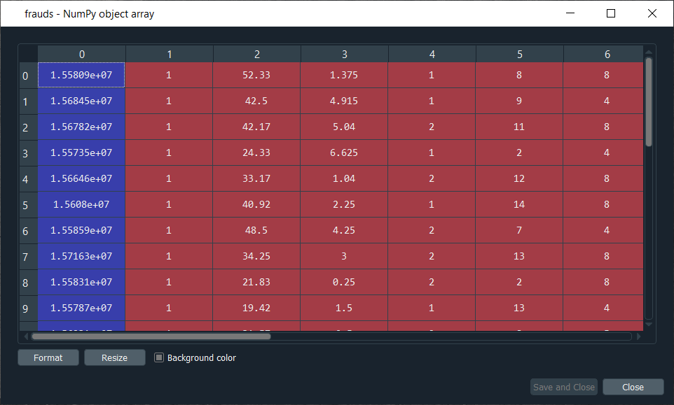
From the above image, it can be seen that we have the customer ID that we can use to find the potential cheaters. So, here we completed our job by giving the list of potential cheaters to the bank. Further, the analyst will investigate the list of potential cheaters for which he will probably get the values of y for all these customer IDs to take in priority the ones that got approved to revise the application and then by investigating deeper, and they will find out if the customer really cheated somehow.
Next TopicMega Case Study
|
 For Videos Join Our Youtube Channel: Join Now
Feedback
- Send your Feedback to [email protected]
Help Others, Please Share


