| |

Restricted Boltzmann MachineNowadays, Restricted Boltzmann Machine is an undirected graphical model that plays a major role in the deep learning framework. Initially, it was introduced by Paul Smolensky in 1986 as a Harmonium, which then gained huge popularity in recent years in the context of the Netflix Price, where RBM achieved state-of-the-art performance in collaborative filtering and have beaten most of the competition. 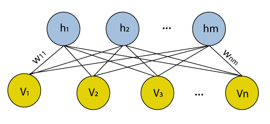
Many hidden layers can be efficiently learned by composing restricted Boltzmann machines using the future activations of one as the training data for the next. These are basically the neural network that belongs to so-called energy-based models. It is an algorithm that is used for dimensionality reduction, classification, regression collaborative filtering, feature learning, and topic modeling. Autoencoders vs. Restricted Boltzmann MachineAutoencoders are none other than a neural network that encompasses 3-layers, such that the output layer is connected back to the input layer. It has much less hidden units in comparison to the visible units. It performs the training task in order to minimize reconstruction or error. In simple words, we can say that training helps in discovering an efficient way for the representation of the input data. 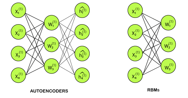
However, RBM also shares a similar idea, but instead of using deterministic distribution, it uses the stochastic units with a particular distribution. It trains the model to understand the association between the two sets of variables. RBM has two biases, which is one of the most important aspects that distinguish them from other autoencoders. The hidden bias helps the RBM provide the activations on the forward pass, while the visible layer biases help the RBM learns the reconstruction on the backward pass. Layers in Restricted Boltzmann MachineThe Restricted Boltzmann Machines are shallow; they basically have two-layer neural nets that constitute the building blocks of deep belief networks. The input layer is the first layer in RBM, which is also known as visible, and then we have the second layer, i.e., the hidden layer. Each node represents a neuron-like unit, which is further interconnected to each other crossways the different layers. 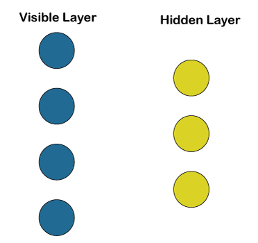
But no two nodes of the same layer are linked, affirms that there is no intralayer communication, which is the only restriction in the restricted Boltzmann machine. At each node, the calculation takes place by simply processing the inputs and makes the stochastic decisions about whether it should start transmitting the input or not. Working of Restricted Boltzmann MachineA low-level feature is taken by each of the visible node from an item residing in the database so that it can be learned; for example, from a dataset of grayscale images, each visible node would receive one-pixel value for each pixel in one image. Let's follow that single pixel value X through the two-layer net. At the very first node of the hidden layer, X gets multiplied by a weight, which is then added to the bias. After then the result is provided to the activation function so that it can produce the output of that node, or the signal's strength, which passes through it when the input x is already given. 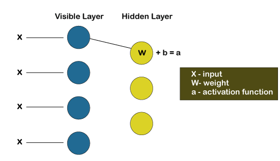
After now, we will look at how different inputs get combines at one particular hidden node. Basically, each X gets multiplied by a distinct weight, followed by summing up their products and then add them to the bias. Again, the result is provided to the activation function to produce the output of that node. 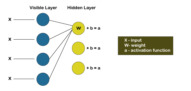
Each of the input X gets multiplied by an individual weight w at each hidden node. In other words, we can say that a single input would encounter three weights, which will further result in a total of 12 weights, i.e. (4 input nodes x 3 hidden nodes). The weights between the two layers will always form a matrix where the rows are equal to the input nodes, and the columns are equal to the output nodes. 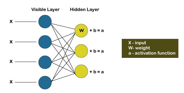
Here each of the hidden nodes is going to receive four inputs, which will get multiplied by the separate weights followed by again adding these products to the bias. Then it passes the result through the activation algorithm to produce one output for each hidden node. Training of Restricted Boltzmann MachineThe training of a Restricted Boltzmann Machine is completely different from that of the Neural Networks via stochastic gradient descent. Following are the two main training steps:
Gibbs sampling is the first part of the training. Whenever we are given an input vector v, we use the following p(h| v) for predicting the hidden values h. However, if we are given the hidden values h, we use p(v| h) to predict the new input values v. 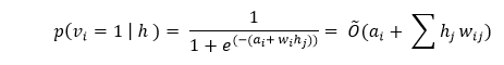
This process is repeated numerously (k times), such that after each iteration (k), we obtain another input vector v_k, which is recreated from the original input value v_0. 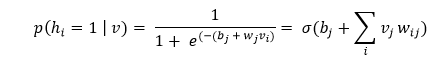
During the contrastive divergence step, it updates the weight matrix gets. To analyze the activation probabilities for hidden values h_0 and h_k, it uses the vector v_0 and v_k. 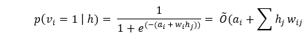
The update matrix is calculated as a difference between the outer products of the probabilities with input vectors v_0 and v_k, which is represented by the following matrix. 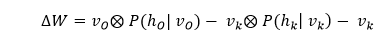
Now with the help of this update weight matrix, we can analyze new weight with the gradient descent that is given by the following equation. 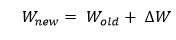
Training to PredictionStep1: Train the network on the data of all the users. Step2: Take the training data of a specific user during inference time. Step3: Use the data to obtain the activations of the hidden neuron. Step4: Use the hidden neuron values to get the activations of the input neurons. Step5: The new values of input neurons show the rating the user would give. Building a Restricted Boltzmann MachineWe are going to implement our Restricted Boltzmann Machine with PyTorch, which is a highly advanced Deep Learning and AI platform. We have to make sure that we install PyTorch on our machine, and to do that, follow the below steps. For Windows users: Click on the Windows button in the Inside the Anaconda prompt, run the following command. 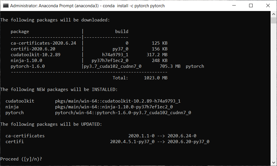
From the above image, we can see that it asks whether to proceed or not. Confirm it with y and press enter. 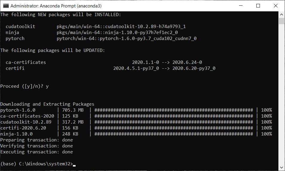
We can see from the above image that we have successfully installed our library. After this, we will move on to build our two recommended systems, one of which will predict if the user is going to like yes/no a movie, and the other one will predict the rating of a movie by a user. So, the first one will predict the binary outcome, 1 or 0, i.e., yes or no, and the second one predicts the rating from 1 to 5. In this way, we will have the most recommended system that is mostly used in the industry. Nowadays, many companies build some recommended systems and most of the time, these recommended systems either predict if the user or the customer is going to like yes or no the product or some other recommended systems can predict a rating or review of certain products. So, we will create the recommended system that predicts a binary outcome yes or no with our restricted Boltzmann machines. The neural network that we will implement in this topic, and then we will implement the other recommended system that predicts the rating from 1 to 5 in the next topic, which is an Autoencoder. However, for both of these recommended systems, we will use the same dataset, which is actually the real-world dataset that can be found online, i.e., MovieLens dataset. You can download the dataset by clicking on the link; https://grouplens.org/datasets/movielens/, which will direct you to the official website. This dataset was created by the grouplens research, and on that page, you will see several datasets with different amounts of ratings. But we will work with older datasets with another 100,000 ratings from 1000 users and 1700 movies, as shown in the image given below. Also, we have another old dataset with one million rates, so I recommend you to have a look at these datasets and download them. Here we are going to download both of the red marked datasets. 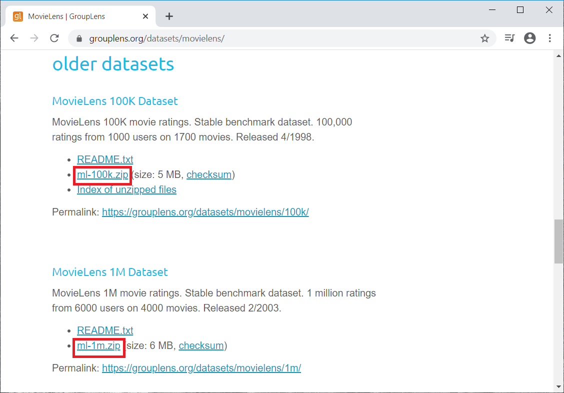
Next, we will import the libraries that we will be using to import our Restricted Boltzmann Machines. Since we will be working with arrays, so we will import NumPy. Then there are Pandas to import the dataset and create the training set and test set. Next, we have all the Torch libraries; for example, nn is the module of Torch to implement the neural network. Here the parallel is for the parallel computations, optim is for the optimizers, utils are the tools that we will use, and autograd is for stochastic gradient descent. After importing all the libraries, classes and functions, we will now import our dataset. The first dataset that we are going to import is all your movies, which are in the file movies.dat. So, we will create new variable movies that will contain all our movies and then we will use the read_csv() function for reading the CSV file. Inside the function, we will pass the following argument:
Output: 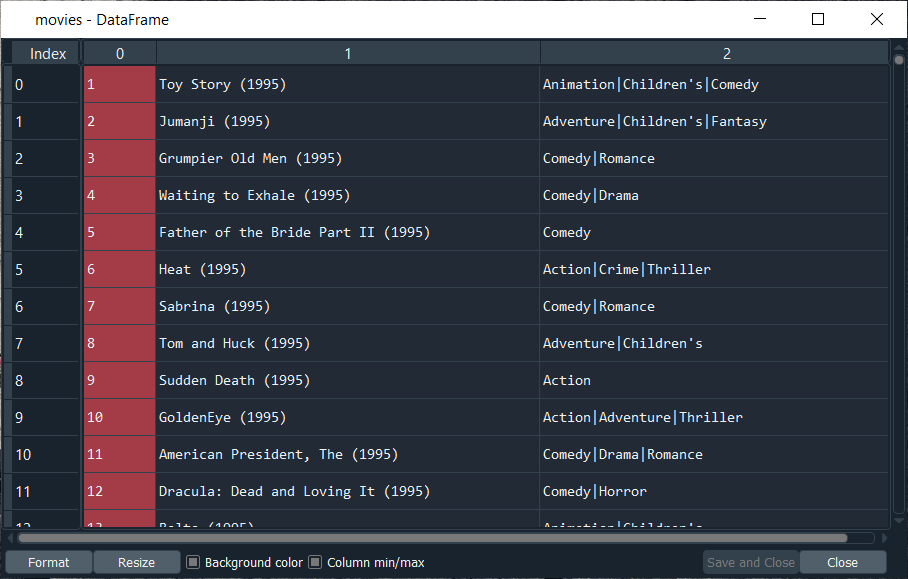
After executing the above line, we will get the list of all the movies in the MovieLens database. We have thousands of movies, and for each of these movies, we have the first column, which is the movie ID, and that's the most important information because we will use it to make our recommended system. We will not use the titles; in fact, it will be much simpler with the movies ID. Next, in the same way, we will import the user dataset. So, we will create a new variable Users for which we will just change the path, and the rest of the things will remain the same because we actually need to use the exact same arguments here for the separator, header, engine, as well as encoding. Output: 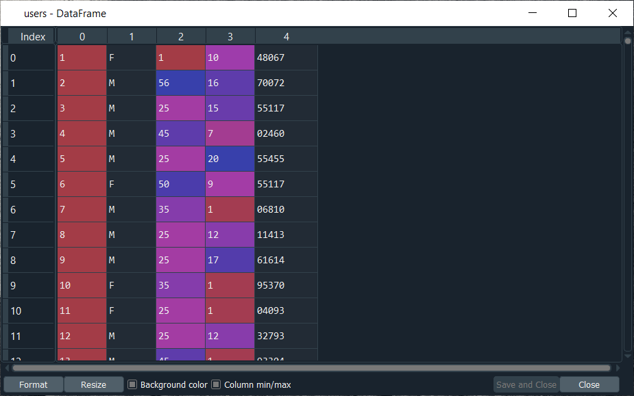
From the above image, we can see that we got all the different information of the users, where the first column is the user ID, the second column is the gender, the third column is the age, the fourth column is some codes that corresponds to the user's job, and lastly the fifth column is the zip code. Now we will import the ratings, which we will do again as we did before just, we will create new variable Ratings followed by changing its path, and the rest will remain the same as it is. Output: 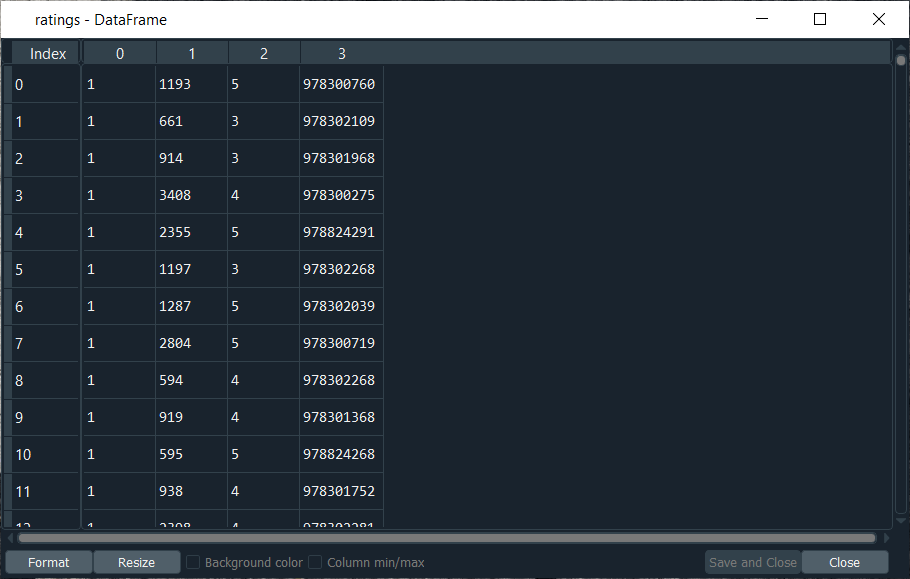
After executing the above line of code, we can see that we have successfully imported our ratings variable. Here the first column corresponds to the users, such that all of 1's corresponds to the same user. Then the second column relates to the movies, and the numbers shown in the second column are the movies ID that is contained in the movies DataFrame. Next, the third column corresponds to the ratings, which goes from 1 to 5. And the last column is the timesteps that specify when each user rated the movie. Next, we will prepare the training set and the test set for which we will create a variable training_set followed by using the Pandas library to import u1.base. Then we will convert this training set into an array because by importing u1.base with Pandas, we will end up getting a DataFrame. So, first, we will use pandas read_csv function, and then we will pass our first argument, which is the path that will take the u1.base in the ml-100k folder and in order to do that, we will start with the folder that contains u1.base, which actually resides in the ml-100k folder followed by adding the name of the training set, i.e., u1.base. Since the separator for the u1.base is the tab instead of the double column, so we need to specify it because otherwise, it will take a comma, which is the default separator. Therefore, we will add our second argument, which is the delimiter = '\t' to specify the tab. As we already saw, the whole original dataset in the ml-100k contains 100,000 ratings, and since each observation corresponds to one rating, we can see from the image given below that after executing the above line of code, we have 80,000 ratings. Therefore, the training set is 80% of the original dataset composed of 100,000 ratings. So, it will be an 80%:20% train: test split, which is an optimal split of the training set and the test set to train a model. 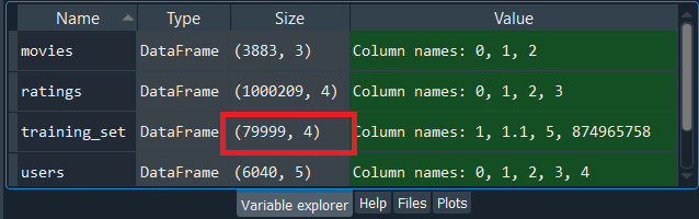
We can check the training_set variable, simply by clicking on it to see what it looks like. Output: 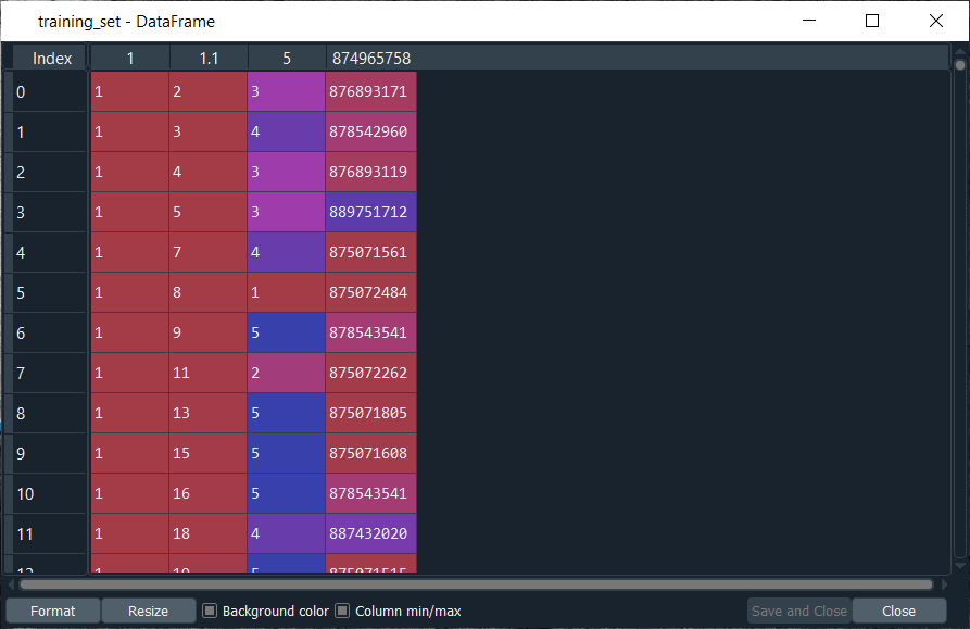
From the above image, we can see that it is exactly the same to that of the ratings dataset that we imported earlier, i.e., the first column corresponds to the users, the second column corresponds to the movies, the third column corresponds to the ratings, and the fourth column corresponds to the timesteps that specifically we really don't need because it won't be relevant to train the model. The training_set is imported as DataFrame, which we have to convert it into an array because later on in this topic, we will be using the PyTorch tensors, and for that, we need an array instead of the DataFrames. After this, we will convert this training set into an array for which we will again take our training_set variable followed by using a NumPy function, i.e., array to convert a DataFrame into an array. Inside the function, we will first input the training_set argument, and as a second argument, we will need to specify the type of this new array that we are creating. Since we only have user IDs, movie IDs and ratings, which are all integers, so we will convert this whole array into an array of integers, and to do this, we will input dtype = 'int' for integers. After executing the above line, we will see that our training_set is as an array of integer32 and of the same size as shown in the below image. 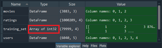
We can check the training_set variable, simply by clicking on it to see what it looks like. Output: 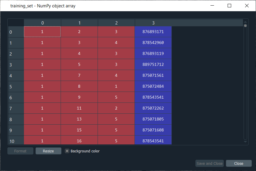
It can be seen from the above image that we got the same values, but this time into an array. Now, in the same way, we will do for the test set, we will prepare the test_set, which will be quite easy this time because we will incorporate the same techniques to import and convert our test_set into an array. We will exactly use the above code. All we got to do is replace the training_set by the test_set as well as u1.base by u1.test because we are taking now the test set, which is u1.test. After executing the above line, we will get our test_set, and we can see that this is exactly the same structure. We have the users in the first column, then the movies in the second column and the ratings in the third column. From the image given below, we have to understand that both the test_set and the training_set have different ratings. There is no common rating of the same movie by the same user between the training_set and the test_set. However, we have the same users. Here indeed, we start with user 1 as in the training_set, but for this same user 1, we won't have the same movies because the ratings are different. Output: 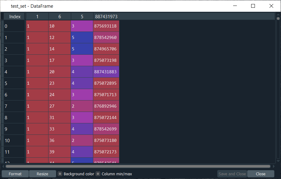
Since our dataset is again a DataFrame, so we need to convert it into an array and to do that, we will do it in the same way as we did for the training_set. After running the above line of code, we can see from the image given below that our test_set is an array of integers32 of 20,000 ratings that correspond to the 20% of the original dataset composed of the 100,000 ratings. 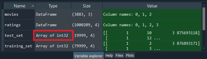
We can check the test_set variable, simply by clicking on it to see what it looks like. Output: 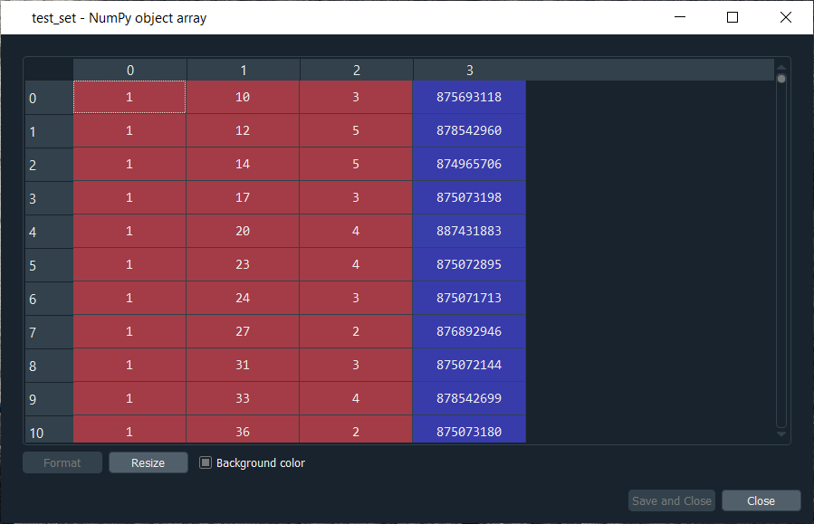
It can be seen from the above image that we got the same values, but this time into an array. In the next step, we are going to get the total number of users and movies because, in the further steps, we will be converting our training_set as well as the test_set into a matrix, where the lines are going to be users, the columns are going to be the movies and the cells are going to be the ratings. We are going to create such a matrix for the training_set and another one for the test_set. However, besides these two matrices, we want to include all the users and all the movies from the original dataset. And if in the training set that we just imported, a user didn't rate a movie, well, in that case, we will put a 0 into the cell of the matric that corresponds to this user and those movies. Therefore, in order to get the total number of users and the total of movies, we will take the maximum of the maximum user ID in the training_set as well as the test_set, so that we can get the total number of users and the total number of movies, which will further help us in making the matrix of users in line and movies in columns. To do this, we will make two new variables, nb_users, which is going to be the total number of users and nb_movies that is going to be the total number of movies. And as we said, we are going to take the max of the maximum user ID in the training set, so we will do with the help of max(max(training_set[:,0]). Inside the brackets, we are required to put the index of the user column, and that is index 0, as well as we needed to take all the lines, so we have added :. Therefore, the training_set[:,0] corresponds to the first column of the training_set, i.e., the users and since we are taking the max, which means we are definitely taking the maximum of the user ID column. After this, we need to do the same for the test_set because the maximum user ID might be in the test set, so in the same manner, we will do for the test set and to do that, we will now take max(test_set[:,0]). In order to force the max number to be an integer, we have to convert the number into an integer, and for that reason, we have used the int function followed by putting all these maximums inside the int function, as shown below. By executing the above line, we will get the total number of user IDs is 943, but it might not work the same way for the other train/test split, so we will use the above code in case we want to apply for the other training and test sets. 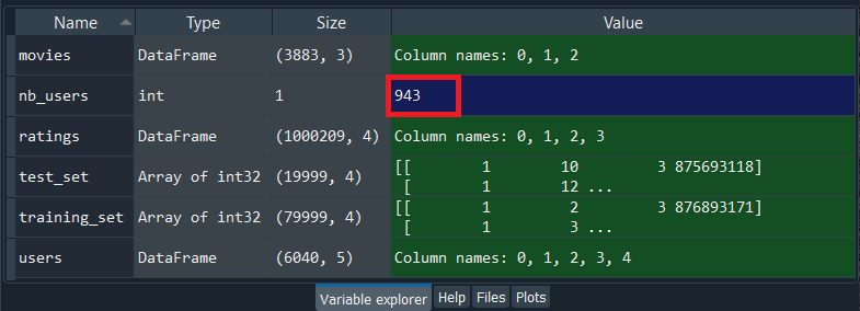
Now, in the same we will do for the movies, we will use the same code but will replace the index of the column users, which is 0 by the index of the column movies, i.e., 1. 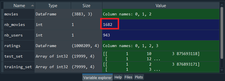
By executing the above line, we get the total number of movie IDs is 1682. So, we had to take the max of the max because we don't know if this movie ID was in the training set or test set, and we actually check out by running the following command. Therefore, the maximum movie ID in the training_set is 1682. 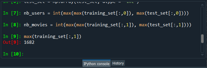
In the same way, we can check for the test_set. After running the above code, we can see from the image given below that the maximum movie ID in the test_set it 1591. So, it could have been in the test_set, which is not the case for this first train/test split, but it could be the other way for other train/test splits. 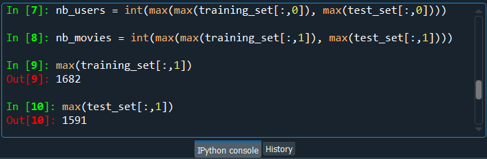
Now we will convert our training_set and test_set into an array with users in lines and movies in columns because we need to make a specific structure of data that will correspond to what the restricted Boltzmann machine expects as inputs. The restricted Boltzmann machines are a type of neural network where you have some input nodes that are the features, and you have some observations going one by one into the networks starting with the input nodes. So, we will create a structure that will contain these observations, which will go into the network, and their different features will go into the input nodes. Basically, we are just making the usual structure of data for neural networks or even for machine learning in general, i.e., with the observation in lines and the features in columns, which is exactly the structure of data expected by the neural network. Thus, we will convert our data into such a structure, and since we are going to do this for both the training_set and the test_set, so we will create a function which we will apply to both of them separately. In order to create a function in python, we will start with def, which stands for definition, followed by giving it a name called convert(). Inside the function, we will pass only one argument, i.e., data because we will apply this function to only a set, which will be the training_set first and then the test_set. Next, we will create a list of lists, which means we will be creating several lists where one list is for each line/user. Since we have 943 users, so accordingly, we will have 943 lists, and these will be horizontal lists, which will correspond to our observations in lines in the special structure that we have just described. The first list will correspond to the first user, the second list will correspond to the second user, etc. and by doing this, we will get the ratings of 1682 movies by the user corresponding to the list. Basically, we will get the ratings for each of the movies where if the user didn't rate the movie, well, in that case, we will get a 0 for that set. This is the reason why the newly converted training_set and the test_set will have the same size because, for both of them, we are considering all the users and all the movies, and we just put 0 when the user didn't rate the movie. So, we will create the list of lists by calling it new_data, which will be our final output that the function will return, i.e., it will be the final array with the users in lines and the movies in the columns. Since the new_data is a list of lists, so we need to initialize it as a list. After this, we will make a loop because we want to create a list for each user, the list of all the ratings of the movies by the user, and therefore, we need a for loop that will get the ratings for each user. In order to make for loop, we will introduce a local variable that will loop over all the users of the data, i.e., the training_set or the test_set. So, we will call this variable as id_users that will take all the IDs of the users in our database followed by specifying a range for these user IDs, which is going to be all the user IDs from one to the max, i.e., the total number of users that we found earlier before initiating this step. Therefore, the id_users will range from 1 to nb_users + 1 so that when it goes up to 944, it will be excluded, and we will go up to 943. Now inside the loop, we will create the first list of this new data list, which is ratings of the first user because here the id_users start at 1, which is why we will start with the first user, and so, we will add the list of ratings of the first user in the whole list. We will get all the movie IDs of all the movies that were rated by the first user, and in order to do this, we will put all the movie IDs into a variable called id_movies. Then we will take our data, which is assumed to be our training_set because then we will apply to convert to the training_set and then from the training set, we will first take the column that contains all the movie IDs, which is 2nd column of our index, i.e., index 1.Next, we will take all the observation for which we will use : followed by separating the colon and the one by the comma, i.e. [:,1]. It basically means that we are only taking the whole column here, the whole one with all the users. Since we only want the movies IDs of the first user because we are at the beginning of the loop, so we will make some kind of syntax that will tell we want the first column of the data, i.e., the training_set such that the first column equals to one and to do this in python, we will add a new condition that we will add in a new pair of brackets []. Inside this bracket, we will put the condition data[:,0] == id_users, which will take all the movies ID for the first user. Now, in the same way, we will get the same for the ratings, i.e., we will get all the ratings of that same first user. Instead of taking id_movies, we will take id_ratings as we want to take all the ratings of the training_set, which is in the 3rd index column, i.e., at index 2, so we will only need to replace 1 by 2, and the rest will remain same. By doing this, we will have all that we needed to create the first list, i.e., is the list of the ratings of the first user. After this, we will get all the zeros when the user didn't rate the movie or more specifically, we can say that we will now create a list of 1682 elements, where the elements of this list correspond to 1682 movies, such that for each of the movie we get the rating of the movie if the user rated the movie and a zero if the user didn't rate the movie. So, we will start with initializing the list of 1682 movies for which we will first call this list as ratings followed by using NumPy that has a shortcut np and then we will use a zeros function. Inside this function, we will put the number of zeros that we want to have in this list, i.e., 1682, which corresponds to nb_movies. After this, we will replace the zeros by the ratings for the movies that the user rated and in order to do this, we will take the ratings followed by adding [id_movies - 1] as it will get us the indexes of the movies that were rated. These indices are the id_movies that we already created in the few steps ago because it contains all the indexes of the movies that were rated, which is exactly what we want to do. Since in python, the indexes start at 0, but in the id_movies, the index starts as 1, and we basically need the movie ID to start at the same base as the indexes of the ratings, i.e., 0, so we have added -1. As we managed to get the indexes of the movies that were rated in the rating list of all the movies, so for these ratings, we will give the real ratings by adding id_ratings. By doing this, we managed to create for each user the list of all the ratings, including the zeros for the movies that were not rated. Now, we are left with only one thing to do, i.e., to add the list of ratings here corresponding to one user to the huge list that will contain all the different lists for all the diffe+rent users. So, we will take this whole list, i.e., new_data, followed by taking the append function as it will append this list of ratings here for one user for the user of the loop, id_users to this whole new_data list. Inside the function, we will put the whole list of ratings for one particular user. And in order to make sure that this is a list, we will put ratings into the list function because we are looking for a list of lists, which is actually expected by PyTorch. So, here we are done with our function, now we will apply it to our training_set and test_set. But before moving ahead, we need to add the final line to return what we want and to do that, we will first add return followed by adding new_data, which is the list of all the different lists of ratings. The next step is to apply this function to the training_set as well as the test_set, and to do this; we will our training_set followed by using the convert function on it. Inside the convert function, we will add the training_set that is the old version of the training_set, which will then become the new version, i.e., an array with the users in lines and the movies in the columns. In the exact same manner, we will now do for the test_set. We will only need to replace the training_set by the test_set, and the rest will remain the same. By running the above section of code, we can see from the below image that the training_set is a list of 943 lists. 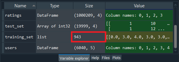
We can also have a look at training_set by simply clicking on it. 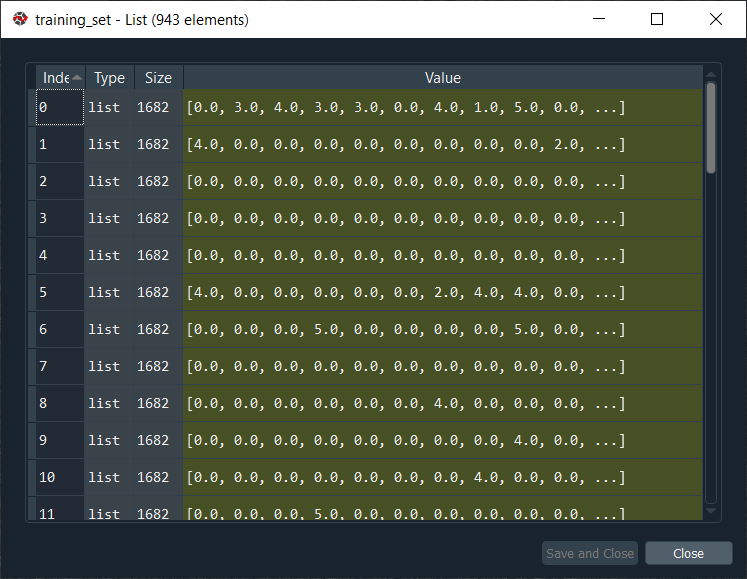
From the above image, we can see this huge list contains 943 horizontal lists, where each of these 943 lists corresponds to each user of our database. So, we can check for the first movie, the second movie and the third movie; the ratings are as expected 0, 3 and 4. It can be clearly seen that for each user, we get the ratings of all the movies of the database, and we get a 0 when the movies weren't rated and the real rating when the user rated the movie. Similarly, for the test_set, we have our new version of test_set that also contains a list of 943 elements, as shown below. 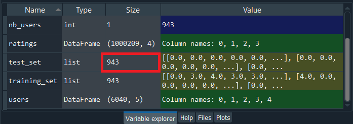
Again, we can also have a look at test_set by simply clicking on it. 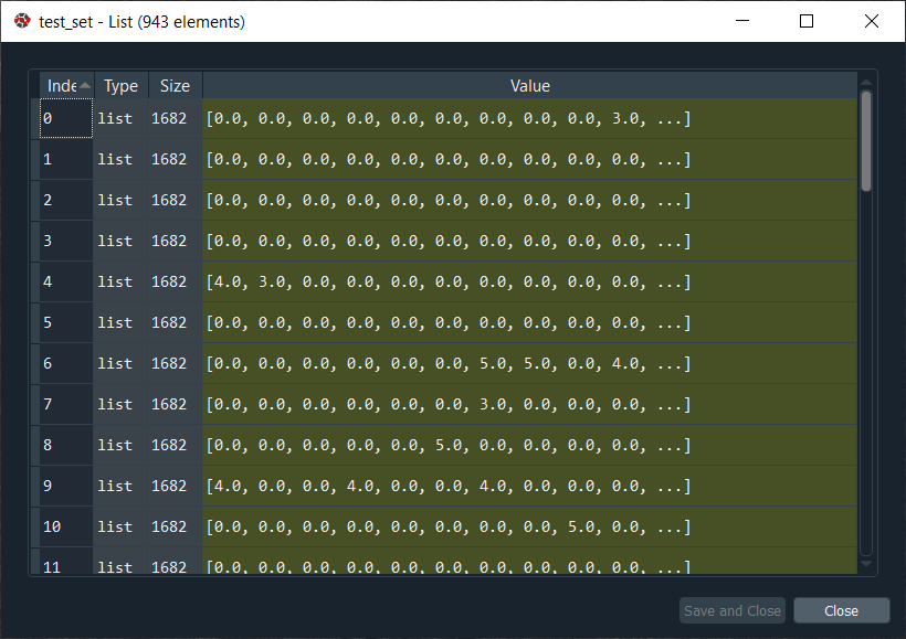
From the above image, we can see that we got a list of lists with all the ratings inside, including 0 for the movies that weren't rated. Next, we will convert our training_set and test_set that are so far a list of lists into some Torch tensors, such that our training_set will be one Torch tensor, and the test_set is going to be another Torch tensor. In a simpler way, we can say that there will be two separate, multi-dimensional matrices based on PyTorch and to do this; we will just use a class from the torch library, which will do the conversion itself. Thus, we will start by taking our training_set, followed by giving it a new value, which will be this converted training set into the torch tensor. So, we will take a torch.FloatTensor, where the torch is the library, and FloatTensor is the class that will create an object of this class. The object will be the Torch tensor itself, i.e., a multi-dimensional matrix with a single type, and since we are using the FloatTensor class, well, in that case, the single type is going to be a float. Inside the class, we will take one argument, which has to be the list of lists, i.e., the training_set, and this is the reason why we had to make this conversion into a list of lists in the previous section because the FloatTensor class expects a list of lists. Similarly, we will do for the test_set. We only need to replace the training_set by the test_set, and the rest will remain the same. After running the below code, we will see that the training_set and the test_set variable will get disappear in the variable explorer pane because, in Spyder, it doesn't recognize the torch tensor yet. However, the variable will still exist, but they will not be displayed in the variable explorer pane. After executing the above two lines of code, our training_set and the test_set variable will get disappear, but they are now converted into a Torch tensor, and with this, we are done with the common data pre-processing for a recommended system. In the next step, we will convert the ratings into binary ratings, 0 or 1, because these are going to be the inputs of our restricted Boltzmann machines. So, we will start with the training_set, and then we will replace all the 0's in the original training set by -1 because all the zeros in the original training_set, all the ratings that were not, actually, existent, these corresponded to the movies that were not rated by the users. In order to access these original ratings that were 0 in the original dataset, we will do this with the help of [training_set == 0] as it will interpret that we want to take all the values of the training_set, such that the values of the training_set are equal to 0. And for all these zero values in the training_set, these zero ratings, we want to replace them by -1. Now we will do for the other ratings as well, i.e., the ratings from 1 to 5. It will be done in the same way as we did above by taking care of ratings that we want to convert into zero, i.e., not liked. As we already discussed, the movies that are not liked by the user are the movies that were given one star or two stars. So, we will do the same for the ratings that were equal to one, simply by replacing 0 by 1 and -1 by 0 because, in our new ratings, format 0 corresponds to the movies that the users didn't like. Again, we will do the same for the ratings that were equal to two in the original training_set. We will now replace 1 by 2, and the rest will remain the same. So, with these two lines given below, all the ratings that were equal to 1 or 2 in the original training_set will now be equal to 0. After this, we simply need to do for the movies that the users liked. So, the movies that were rated at least three stars were rather liked by the users, which means that the three stars, four stars and five stars will become 1. In order to access the three, four and five stars, we need to replace == by >= to include 3 and not the 2. So, [training_set >= 3] means that all the values in the training_set larger or equal to three will include getting the rating, 1. By doing this, three, four and five will become one in the training_set. Since we want the RBM to output the ratings in binary format, so the inputs must have the same binary format 0 or 1, which we successfully converted all our ratings in the training_set. Now we will do the same for the test_set, and to do this, we will copy the whole above code section and simply replace all the training_set by the test_set. So, with this, all the ratings from 1 to 5 will be converted into the binary ratings in both the training_set and the test_set. After executing the above section of code, our inputs are ready to go into the RBM so that it can return the ratings of the movies that were not originally rated in the input vector because this is unsupervised deep learning, and that's how it actually works. Now we will create the architecture of the Neural Network, i.e., the architecture of the Restricted Boltzmann Machines. So, we will choose the number of hidden nodes, and mostly we will build the neural network just like how it works, i.e., we will make this probabilistic graphical model because an RBM is itself a probabilistic graphical model and to build it, we will use class. Basically, we will make three functions; one to initialize the RBM object that we will create, the second function will be sample H that will sample the probabilities of the hidden nodes given the visible nodes, and the third function will be sample V, which will sample the probabilities of the visible nodes given the hidden nodes. So, we will start with defining the class by naming it as RBM, and inside the class, we will first make the __init__() function that defines the parameters of the object that will be created once the class is made. It is, by default, a compulsory function, which will be defined as def __init__(). After this, we will input the following arguments inside the function:
Since we want to initialize the weight and bias, so we will go inside the function where we will initialize the parameters of our future objects, the object that we will create from this class. Basically, inside the __init__ function, we will initialize all the parameters that we will optimize during the training of the RBM, i.e., the weights and the bias. And since these parameters are specific to the RBM model, i.e., to our future objects that we are going to create from the RBM class, so we need to specify these variables are the variables of the object. Therefore, to initialize these variables, we need to start with self.W, where W is the name of the weight variable. These weights are all the parameters of the probabilities of the visible nodes given the hidden nodes. Next, we will use the torch, the torch library, followed by using the randn function to randomly initialize all the weights in tensor, which should be of size nh and nv. Next, we will initialize the bias. There is some bias for the probability of the hidden node given the visible node and some bias for the probability of the visible node given the hidden node. So, we will start with the bias for the probabilities of the hidden nodes given the visible nodes. It is the same as what we have done before, we will give a name to these biases, and for the first bias, we will name it a. But before that, we will take the self-object because a is the parameter of the object. Then we will again take the torch.randn to initialize the weights according to the normal distribution of mean 0 and variance 1. Since there is only one bias for each hidden node and we have nh hidden nodes, so we will create a vector of nh elements. But we need to create an additional dimension corresponding to the batch, and therefore this vector shouldn't have one dimension like a single input vector; it should have two dimensions. The first dimension corresponding to the batch, and the second dimension corresponding to the bias. So, inside the function, we will first input 1 and then nh as it will help in creating our 2-Dimensional tensor. Then we have our third parameter to define, which is still specific to the object that will be created, which is the bias for the visible nodes, so we will name it as b. Here it is exactly similar to the previous line; we will take the torch.randn function but this time for nv. So, we ended up initializing a tensor of nv elements with one additional dimension corresponding to the batch. Next, we will make the second function that we need for our RBM class, which is all about sampling the hidden nodes according to the probabilities P(h) given v, where h is the hidden node, and v is a visible node. This probability is nothing else than the sigmoid activation function. During the training, we will approximate the log-likelihood gradient through Gibbs sampling, and to apply it, we need to compute the probabilities of the hidden nodes given the visible nodes. Then once we have this probability, we can sample the activations of the hidden nodes. So, we will start by calling our sample_h() to return some samples of the different hidden nodes of our RBM. Inside the sample_h(), we will pass two arguments;
Now, inside the function, we will first compute the probability of h given v, which is the probability that the hidden neurons equal one given the values of the visible neurons, i.e., input vectors of observations with all the ratings. The probability of h given v is nothing but the sigmoid activation function, which is applied to wx, the product of w the vector of weights times x the vector of visible neurons plus the bias a because a corresponds to bias of the hidden nodes. Then b corresponds to the bias of the visible nodes, which we will use to define the sample function, but for the visible nodes. And since we are dealing with hidden nodes at present, so we will take the bias of the hidden nodes, i.e., a. We will start by first computing the product of the weights times the neuron, i.e., x. So, we will first define wx as a variable, and then we will use a torch because we are working with the torch tensors. And since we are about to make a product of two tensors, so we have to take a torch to make that product, for which we will use mm function. Inside the function, we will input our two matrices; matrix 1 and matrix 2. As we said earlier that we want to make the product of x, the visible neurons and nw, the tensor of weights. But here, W is attached to the object because it's the tensor of weights of the object that will be initialized by __init__ function, so instead of taking only W, we will take self.W that we will input inside the mm function. In order to make it mathematically correct, we will compute its transpose of the matrix of weights with the help of t(). After this, we will compute what is going to be inside the sigmoid activation function, which is nothing but the wx plus the bias, i.e., the linear function of the neurons where the coefficients are the weights and then we have the bias, a. We will call the wx + a as an activation because that is what is going to be inside the activation function. Then we will take the wx plus the bias, i.e., a, and since it is attached to the object that will be created by the RBM class, so we need to take self.a to specify that a is the variable of the object. As said previously that each input vector will not be treated individually, but inside the batches and even if the batch contains one input vector or one vector of bias, well that input vector still resides in the batch, we will call it as a mini-batch. So, when we add a bias of the hidden nodes, we want to make sure that this bias is applied to each line of the mini-batch, i.e., of each line of the dimension. We will use the expand_as function that will again add a new dimension for these biases that we are adding, followed by passing wx as an argument inside the function as it corresponds to what we want to expand the bias. Next, we will compute the activation function for which we will call p_h_given_v function, which corresponds to the probability that the hidden node is activated, given the value of the visible node. Since we already discussed that p_h_given_v is the sigmoid of the activation, so we will pursue taking the torch.sigmoid function, followed by passing activation inside the function. After this, in the last step, we will return the probability as well as the sample of h, which is the sample of all the hidden nodes of all the hidden neurons according to the probability p_h_given_v. So, we will first use return p_h_given_v, which will return the first element we want and then torch.bernoulli(p_h_given_v) that will result in returning all the probabilities of the hidden neurons, given the values of the visible nodes, i.e., the ratings as well as the sampling of hidden neurons. So, we just implemented the sample_h function to sample the hidden nodes according to the probability p_h_given_v. We will now do the same for visible nodes because from the values in the hidden nodes, i.e., whether they were activated or not, we will also estimate the probabilities of the visible nodes, which are the probabilities that each of the visible nodes equals one. In the end, we will output the predicted ratings, 0 or 1 of the movies that were not originally rated by the user, and these new ratings that we get in the end will be taken from what we obtained in the hidden node, i.e., from the sample of the hidden node. Thus, we will make the function sample_v because it is also required for Gibbs sampling that we will apply when we approximate the log-likelihood gradient. And in order to make this function, it is exactly the same as that of the above function; we will only need to replace few things. First, we will call the function sample_v because we will make some samples of the visible nodes according to the probabilities p_v_given_h, i.e., given the values of the hidden nodes, we return the probabilities that each of the visible nodes equals one. Here we will return the p_v_given_h and some samples of the visible node still based on the Bernoulli sampling, i.e., we have our vector of probabilities of the visible nodes, and from this vector, we will return some sampling of the visible node. Next, we will change what's inside the activation function, and to that, we will first replace variable x by y because x in the sample_h function represented the visible node, but here we are making the sample_v function that will return the probabilities of the visible nodes given the values of hidden nodes, so the variable is this time the values of the hidden nodes and y corresponds to the hidden nodes. Similarly, we will replace wx by wy, and then we take the torch product of matrices of tensors of not x but y by the torch tensor of all the weights. Since we are making the product of the hidden nodes and the torch tensor of weight, i.e., W for the probabilities p_v_given_h, so we will not take the transpose here. After this, we will compute the activation of the hidden neurons inside the sigmoid function, and for that, we will not take wx but wy as well as we will replace a by b for the fact that we will need to take the bias of the visible node, which is contained in self.b variable, keeping the rest remain same. Now we will make our last function, which is about the contrastive divergence that we will use to approximate the log-likelihood gradient because the RBM is an energy-based model, i.e., we have some energy function which we are trying to minimize and since this energy function depends on the weights of the model, all the weights in the tensor of weights that we defined in the beginning, so we need to optimize these weights to minimize the energy. Not that it can be seen as an energy-based model, but it can also be seen as a probabilistic graphical model where the goal is to maximize the log-likelihood of the training set. In order to minimize the energy or to maximize the log-likelihood for any deep learning model or a machine learning model, we need to compute the gradient. However, the direct computations of the gradient are too heavy, so instead of directly computing it, we will rather try to approximate the gradient with the help of Contrastive Divergence. So, we will again start with defining our new function called a train, and then inside the function, we will pass several arguments, which are as follows:
After this, we will take our tensor or weights self.W, and since we have to take it again and add something, so we will take +=. Then we will make the product of the probabilities that the hidden nodes equal one given the input vector v0 by that input vector v0 and the probability that the hidden node equals one given the input vector v0 is nothing else than ph0. Thus, in order to do that, we will first take our torch library followed by mm to make the product of two tensors, and within the parenthesis, we will input the two tensors in that product, i.e., v0, the input vector of observations followed by taking its transpose with the help of t() and then ph0, which is the second element of the product. Then we will need to subtract again torch.mm, the torch product of the visible nodes obtained after k sampling, i.e., vk followed by taking its transpose with the help of t() and the probabilities that the hidden nodes equal one given the values of these visible nodes vk, which is nothing else than phk. Next, we will update the weight b, which is the bias of the probabilities p(v) given h and in order to do that, we will start by taking self.b and then again += because we will be adding something to b followed by taking torch.sum as we are going to sum (v0 - vk), which is the difference between the input vector of observations v0 and the visible nodes after k sampling vk and 0. Basically, we are just making the sum of v0-vk and 0, which is just to keep the format of b as a tensor of two dimensions. After this, we will do our last update, i.e., bias a that contains the probabilities of P(h) given v. So, we will start with self.a followed by taking += because we will be adding something as well, i.e., we will add the difference between the probabilities that the hidden node equals one given the value of v0, the input vector of observations and the probabilities that the hidden nodes equals one given the value of vk, which is the value of the visible nodes after k sampling. Basically, we will just add the difference (ph0-phk) and 0, which we will perform in the same way as we did just above. Now we have our class, and we can use it to create several objects. So, we can create several RBM models. We can test many of them with different configurations, i.e., with several number of hidden nodes because that is our main parameter. But then we can also add some more parameters to the class like a learning rate in order to improve and tune the model. After executing the above sections of code, we are now ready to create our RBM object for which we will need two parameters, nv and nh. Here nv is a fixed parameter that corresponds to the number of movies because nv is the number of visible nodes, and at the start, the visible nodes are the ratings of all the movies by a specific user, which is the only reason we have one visible node for each movie. So, we have a number of ways to get the number of visible nodes; first, we can say nv equals to nb_movies, 1682 or the other way is to make sure that it corresponds to the number of features in our matrix of features, which is the training set, tensor of features. Therefore, we will start by defining nv as len(training_set[0]), where training_set[0] corresponds to the first line of the training set and len(training_set[0]) is the number of elements in the first line, i.e., the number of features we want for nv. Next, we will do for nh, which corresponds to the number of hidden nodes. Since we have 1682 movies, or we can say 1682 visible nodes, and as we know, the hidden nodes correspond to some features that are going to be detected by the RBM model, so initially, we will start by detecting 100 features. Then we have another variable, batch_size, which was not highlighted yet. However, we already mention its concept in the above code section, and that is because when we train our model algorithm, we will not update the weights after each observation rather, we will update the weights after several observations that will go into a batch and so the batches will have each one the same number of observations. So, this additional parameter that we can tune as well to try to improve the model, in the end, is the batch_size itself. In order to get fast training, we will create a new variable batch_size and make it equal to 100, but you can try with several batch_sizes to have better performance results. Now we will create our RBM object because we have our two required parameters of the __init__ method, i.e., nv and nh. In order to create our object, we will start by calling our object as rbm, followed by taking our class RBM. Inside the class, we will input nv and nh as an argument. Next, we will move on to training our Restricted Boltzmann Machines for which we have to include inside of a for loop, the different functions that we made in the RBM class. We will start by choosing a number of epochs for which we will call the variable nb_epoch followed by making it equal to 10 because we have few observations, i.e., 943 and besides, we only have a binary value 0 and 1, therefore the convergence will be reached pretty fast. After this, we will make a for loop that will go through the 10 epochs. In each epoch, all our observations will go back into the network, followed by updating the weights after the observations of each batch passed through the network, and then, in the end, we will get the final visible node with the new ratings for the movies that were not originally rated. In order to make the for loop, we will start with for then we will come up with a variable for epoch, so we will simply call it as an epoch, which is the name of the looping variable in range and then inside the parenthesis, we will start with (1, nb_epoch+1) that will make sure we go from 1 to 10 because even if nb_epoch + 1 equals to 11, it will not include the upper bound. Then we will go inside the loop and make the loss function to measure the error between the predictions and the real ratings. In this training, we will compare the predictions to the ratings we already have, i.e., the ratings of the training_set. So, basically, we will measure the difference between the predicted ratings, i.e., either 0 or 1 and the real ratings 0 or 1. For this RBM model, we will go with the simple difference in the absolute value method to measure the loss. Thus, we will introduce a loss variable, calling it as train_loss, and we will initialize it to 0 because before starting the training, the loss is zero, which is will further increase when we find some errors between the predictions and the real ratings. After this, we will need a counter because we are going to normalize the train_loss and to normalize the train_loss, we will simply divide the train_loss by the counter, s followed by initializing it to 0. Since we want it to be a float, so we will add a dot after 0 that will make sure s has a float type. And with this, we have a counter, which we will increment after each epoch. Next, we will do the real training that happens with the three functions that we created so far in the above steps, i.e., sample _h, sample_v and train when we made these functions was regarding one user, and of course, the samplings, as well as the contrastive divergence algorithm, have to be done overall users in the batch. Therefore, we will first get the batches of users, and in order to do that, we will need another for loop. Here we are going to make a for loop inside the first for loop, so will start with for and since this for loop is about looping over all the users, we will introduce a looping variable id_user in range(). As we already know, the indexes of the users start at 0, so we will start the range with 0. Now before we move ahead, one important point is to be noted that we want to take some batches of users. We don't want to take each user one by one and then update the weights, but we want to update the weight after each batch of users going through the network. Therefore, we will not take each user one by one, but we will take the batches of the users. Since the batch_size equals 100, well, the first batch will contain all the users from index 0 to 99, then the second batch_size will contain the users from index 100 to index 199, and the third batch_size will be from 200 to 299, etc. until the end. So, the last batch that will go into the network will be the batch_size of the users from index 943 - 100 = 84, which means that the last batch will contain the users from 843 to 943. Hence the stop of the range for the user is not nb_users but nb_users - batch_size, i.e., 843. After this, we will need a step because we don't want to go from 1 to 1, instead, we want to go from 1 to 100 and 100 to 200, etc. until the last batch. Thus, the step, which is the third argument that we need to input, will not be 1, the default step but 100, i.e., the batch_size. Now we will get inside the loop, and our first step will be separating out the input and the target, where the input is the ratings of all the movies by the specific user we are dealing in the loop and the target is going to be at the beginning the same as the input. Since the input is going to be inside the Gibbs chain and will be updated to get the new ratings in each visible node, so the input will get change, but the target will remain the same. Therefore, we will call the input as vk because it is going to be the output of the Gibbs sampling after the k steps of the random walk. But initially, this vk will actually be the input batch of all the observations, i.e., the input batch of all the ratings of the users in the batch. So, the input is going to be the training_set, and since we are dealing with a specific user that has the ID id_user, well the batch that we want to get is all the users from id_user up to id_user + batch_size and in order to that, we will [id_user:id_user+batch_size] as it will result in the batch of 100 users. Similarly, we will do for the target, which is the batch of the original ratings that we don't want to touch, but we want to compare it in the end to our predicted ratings. We need it because we want to measure the error between the predicted ratings and the real ratings to get the loss, the train_loss. So, we will call the target as v0, which contains the ratings of the movies that were already rated by the 100 users in this batch. And since the target is the same as the input at the beginning, well, we will just copy the above line of code because, at the beginning, the input is the same as that of the target, it will get updated later on. Then we will take ph0 followed by adding ,_in order to make it understand that we only want to return the first element of the sample_h function. Since sample_h is the method of RBM class, so we will use the sample_h function from our rbm object with the help of rbm.sample_h. Inside the function, we will input v0 as it corresponds to the visible nodes at the start, i.e., the original ratings of the movies for all the users of our batch. In the next step, we will add another for loop for the k steps of contrastive divergence. So, we will start with for followed by calling the looping variable, i.e., k in range(10) Next, we will take _,hk that is going to be the hidden nodes obtained at the kth step of contrastive divergence and as we are at the beginning, so k equals 0. But the h0 is going to be the second element returned by the sample_h method, and since the sample_h method is in the RBM class, so we will call it from our rbm.sample_h. As we are doing the sampling of the first hidden nodes, given the values of the first visible nodes, i.e., the original ratings, well the first input of the sample_h function in the first step of the Gibbs sampling will be vk because vk so far is our input batch of observations and then vk will be updated. Here vk equals v0. Now we will update the vk so that vk is no longer v0, but now vk is going to be the sampled visible nodes after the first step of Gibbs Sampling. In order to get this sample, we will be calling the sample_v function on the first sample of our hidden nodes, i.e., hk, the result of the first sampling based on the first visible nodes, the original visible nodes. Thus, vk is going to be rbm.sample_v that we call on hk, the first sampled hidden nodes. In the next step, we will update the weights and the bias with the help of vk. But before moving ahead, we need to do one important thing. i.e., we will skip the sales that have -1 ratings in the training process by freezing the visible nodes that contain -1 ratings because it would not be possible to update them during the Gibbs sampling. In order to freeze the visible nodes containing the -1 ratings, we will take vk, which is our visible nodes that are being updated during the k-steps of the random walk. Then we will get the nodes that have -1 ratings with the help of our target, v0 because it was not changed, it actually keeps the original ratings. So, we will take [v0<0] to get the -1 ratings due to the fact that our ratings are either -1, 0 or 1. For these visible nodes, we will say that they are equal to -1 ratings by taking the original -1 ratings from the target because it is not changed and to do that, we will take v0[v0<0] as it will get all the -1 ratings. It is just to make sure that the training is not done on these ratings that were not actually existent. We only want to do the training on the ratings that happened. Next, we will compute the phk before applying the train function, and to do this, we will start by taking the phk,_ because we want to get the first element returned by the sample_h function. Then we will get the sample_h function applied on the last sample of the visible nodes, i.e., at the end of for loop. So, we will first take our rbm object followed by applying sample_h function to the last sample of visible nodes after 10 steps, i.e., vk. After now, we will apply the train function, and since it doesn't return anything, so we will not create any new variable, instead, we will our rbm object as it is a function from the RBM class. Then from the rbm object, we will call our train function followed by passing v0, vk, ph0 and phk as an argument inside the function. Now the training will happen easily as well as the weights, and the bias will be updated towards the direction of the maximum likelihood, and therefore, all our probabilities P(v) given the states of the hidden nodes will be more relevant. We will get the largest weights for the probabilities that are the most significant, and will eventually lead us to some predicted ratings, which will be close to the real ratings. Next, we will update the train_loss, and then we will use += because we want to add the error to it, which is the difference between the predicted ratings and the real original ratings of the target, v0. So, we will start by comparing the vk, which is the last of the last visible nodes after the last batch of the users that went through the network to v0, the target that hasn't changed since the beginning. Here we will measure the errors with the help of simple distance in absolute values between the predictions and the real ratings, and to do so, we will use torch function, i.e., mean. Inside the mean function, we will use another torch function, which is the abs function that returns the absolute value of a number. So, we will take the absolute value of the target v0 and our prediction vk. In order to improve the absolute value v0-vk, we will include the ratings for the ones that actually existed, i.e. [v0>=0] for both v0 and vk as it corresponds to the indexes of the ratings that are existent. Now we will update the counter for normalizing the train_loss. So, here we will increment it by 1 in the float. Lastly, we will print all that is going to happen in training, i.e., the number of epochs to see in which epoch we are during the training, and then for these epochs, we want to see the loss, how it is decreasing. So, we will use the print function, which is included in the for loop, looping through all the epochs because we want it to print at each epoch. Inside the print function, we will start with a string, which is going to be the epoch, i.e. 'epoch: ' followed by adding + to concatenate two strings and then we will add our second string that we are getting with the str function because inside this function, we will input the epoch we are at in training, i.e., an integer epoch that will become string inside the str function, so we will simply add str(epoch). Then we will again add + followed by adding another string, i.e. ' loss: ' and then again, we will add + str(train_loss/s). Basically, it will print the epoch where we are at in the training and the associated loss, which is actually the normalized train_loss. So, after executing the above section of code, we can see from the image given below that we ended with a train_loss of 0.245 or we can say 0.25 approximately, which is pretty good because it means that in the training set, we get the correct predictive rating, three times out of four and one times out of four we make a mistake when predicting the ratings of the movies by all the users. 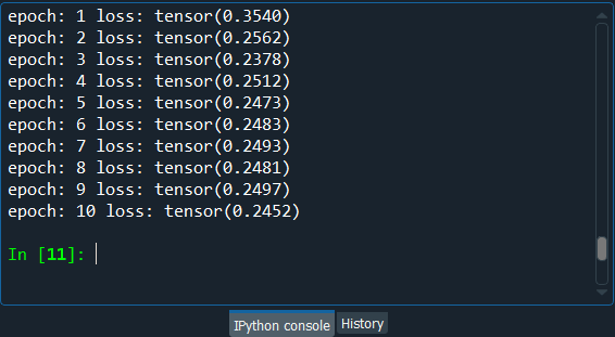
Next, we will get the final results on the new observations with the test_set results so as to see if the results are close to the training_set results, i.e., even on new predictions, we can predict three correct ratings out of four. Testing the test_set result is very easy and quite similar to that of testing the training_set result; the only difference is that there will not be any training. So, we will simply copy the above code and make the required changes. In order to get the test_set results, we will replace the training_set with the test_set. And since there isn't any training, so we don't need the loop over the epoch, and therefore, we will remove nb_epoch = 10, followed by removing the first for loop. Then we will replace the train_loss by the test_loss to compute the loss. We will keep the counter that we initialize at zero, followed by incrementing it by one at each step. Then we have the for loop over all the users of the test_set, so we will not include the batch_size because it is just a technique to specific to the training. It is a parameter that you can tune to get more or less performance results on the training_set and, therefore, on the test_set. But gathering the observations in the batch_size is only for the training phase. Thus, we will remove everything that is related to the batch_size, and we will take the users up to the last user because, basically, we will make some predictions for each user one by one. Also, we will remove 0 because that's the default start. So, we will do for id_user in range(nb_user) because basically, we are looping over all the users, one by one. Now for each user, we will go into the loop, and we will again remove the batch_size because we don't really need them. Since we are going to make the predictions for each user one by one, so we will simply replace the batch_size by 1. After this, we will replace vk by v and v0, which was the target by vt. Here v is the input on which we will make the prediction. For v, which is the input, we will not replace the training_set here by the test_set because the training_set is the input that will be used to activate the hidden neurons to get the output. Since vt contains the original ratings of the test_set, which we will use to compare to our predictions in the end, so we will replace the training_set here with the test_set. Now, we will move on to the next step in which we will make one step so that our prediction will be directly the result of one round trip of Gibbs sampling, or we can say one step, one iteration of the bind walk. Here we will simply remove the for a loop because we don't have to make 10 steps, we only have to make one single step. So, to make this one step, we will start with the if condition to filter the non-existent ratings of the test_set followed by taking the len function. Inside the function, we will input vt[vt>=0], which relates to all the ratings that are existent, i.e. 0 or 1. So if len, the length that is the number of the visible nodes containing set ratings, (vt[vt>=0]) is larger than 0, then we can make some predictions. Since we only have to make one step of the blind walk, i.e., the Gibbs sampling, because we don't have a loop over 10 steps, so we will remove all the k's. Next, we will replace the train_loss by the test_loss in order to update it. And then again, we will update the mean function from the torch library as well as we will still take the absolute distance between the prediction and the target. So, this time, our target will not be v0 but vt, followed by taking all the ratings that are existent in the test_set, i.e. [vt>=0]. Also, the prediction will not vk anymore, but v because there is only step, and then we will again take the same existent ratings, [vt>=0] because it will help us to get the indexes of the cells that have the existent ratings. After now, we will update the counter in order to normalize the test_loss. Lastly, we will print the final test_loss for which we will get rid of all the epochs from the code. Then from the first string, we will replace the loss by the test_loss to specify that it is a test loss. Next, we will replace the train_loss by the test_loss that we divide by s to normalize. Output: 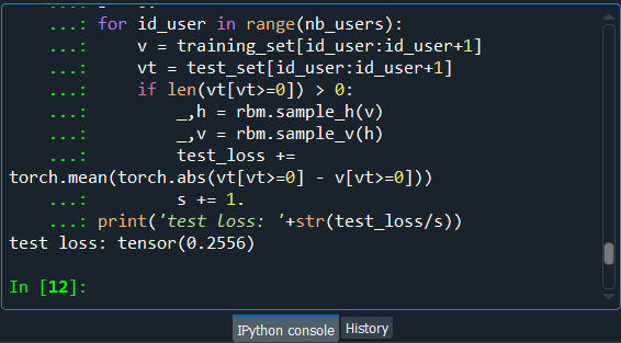
Thus, after executing the above line of code, we can see from the above image that we get a test_loss of 0.25, which is pretty good because that is for new observations, new movies. We managed to predict some correct ratings three times out of four. We actually managed to make a robust recommended system, which was the easier one, predicting the binary ratings.
Next Topic#
|
 lower-left corner -> List of programs -> Anaconda -> Anaconda prompt.
 For Videos Join Our Youtube Channel: Join Now
Feedback
- Send your Feedback to [email protected]
Help Others, Please Share


