PySpark RDD(Resilient Distributed Dataset)In this tutorial, we will learn about building blocks of PySpark called Resilient Distributed Dataset that is popularly known as PySpark RDD. As we have discussed in PySpark introduction, Apache Spark is one of the best frameworks for the Big Data Analytics. This technology becomes more effective and easier when it integrated with Python. It provides us extremely handy and easy to use API called PySpark. What are PySpark RDDs? RDDs are most essential part of the PySpark or we can say backbone of PySpark. It is one of the fundamental schema-less data structures, that can handle both structured and unstructured data. It makes in-memory data sharing 10 - 100x faster in comparison of network and disk sharing. 
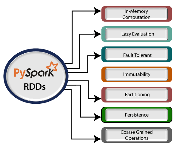
"Resilient Distributed Datasets (RDD) is a distributed memory abstraction that helps a programmer to perform in-memory computations on large cluster." One of the important advantages of RDD is fault tolerance, it means if any failure occurs it recovers automatically. RDD divides data into smaller parts based on a key. The benefit of dividing data into smaller chunks is that if one executor node fails, another node will still process the data. These are able to recover quickly from any issues as the same data chunks are replicated across multiple executor nodes. It provides the functionality to perform functional calculation against dataset very quickly by binding the multiple nodes. RDD becomes immutable when it is created. Immutable mean, we cannot modify an object once it created, but it can surely be transforme. Features of RDDVarious features of PySpark RDDs are following: 
PySpark provides provision of in-memory computation. Computed results are stored in distributed memory (RAM) instead of stable storage (disk). It provides very fast computation
Transformation in PySpark RDDs is lazy. It doesn't compute the result immediately means that execution does not start until an action is triggered. When we call some operation in RDD for transformation, it does not execute immediately. Lazy Evolution plays an important role in saving calculation overhead. It provides the optimization by reducing the number of queries.
RDDs track data lineage information to reconstruct lost data automatically. If failure occurs in any partition of RDDs, then that partition can be re-computed from the original fault tolerant input dataset to create it.
The created data can be retrieved anytime but its value can't be changed. RDDs can only be created through deterministic operations.
RDDs are the collection of various data items that are so huge in size. Because of its size they cannot fit into a single node and must be partitioned across various nodes.
It is an optimization technique where we can save the result of RDD evaluation. It stores the intermediate result so that we can use it further if required. It reduces the computation complexity.
The coarse grained operation means that we can transform the whole dataset but not individual element on the dataset. On the other hand, fine grained mean we can transform individual element on the dataset. Create RDDsPySpark provides two methods to create RDDs: loading an external dataset, or distributing a set of collection of objects. We can create RDDs using the parallelize() function which accepts an already existing collection in program and pass the same to the Spark Context. It is the simplest way to create RDDs. Consider the following code:
Output: +----+----+----+-----+ |col1|col2|col3| col4| +----+----+----+-----+ | 12| 20| 35|a b c| | 41| 58| 64|d e f| | 70| 85| 90|g h i| +----+----+----+-----+
Output: The above code will give the following RDD data. +--------+------+----------+----------+ |Roll_Num| Name|Percentage|Department| +--------+------+----------+----------+ | 009001| Anuj| 70%|B.tech(cs)| | 009002|Sachin| 80%|B.tech(cs)| | 008005|Yogesh| 94%| MCA| | 007014|Ananya| 98%| MCA| +--------+------+----------+----------+
Here we read dataset from .csv file using the read() function. Output: +---+--------------------+-------------+--------------+----------------+------+------------+--------------+--------+--------+-------+--------------+------------+----------+ |_c0| Track.Name| Artist.Name| Genre|Beats.Per.Minute|Energy|Danceability|Loudness..dB..|Liveness|Valence.|Length.|Acousticness..|Speechiness.|Popularity| +---+--------------------+-------------+--------------+----------------+------+------------+--------------+--------+--------+-------+--------------+------------+----------+ | 1| Se?orita| Shawn Mendes| canadian pop| 117| 55| 76| -6| 8| 75| 191| 4| 3| 79| | 2| China| Anuel AA|reggaeton flow| 105| 81| 79| -4| 8| 61| 302| 8| 9| 92| | 3|boyfriend (with S...|Ariana Grande| dance pop| 190| 80| 40| -4| 16| 70| 186| 12| 46| 85| | 4|Beautiful People ...| Ed Sheeran| pop| 93| 65| 64| -8| 8| 55| 198| 12| 19| 86| | 5|Goodbyes (Feat. Y...| Post Malone| dfw rap| 150| 65| 58| -4| 11| 18| 175| 45| 7| 94| +---+--------------------+-------------+--------------+----------------+------+------------+--------------+--------+--------+-------+--------------+------------+----------+ only showing top 5 rows root |-- _c0: integer (nullable = true) |-- Track.Name: string (nullable = true) |-- Artist.Name: string (nullable = true) |-- Genre: string (nullable = true) |-- Beats.Per.Minute: integer (nullable = true) |-- Energy: integer (nullable = true) |-- Danceability: integer (nullable = true) |-- Loudness..dB..: integer (nullable = true) |-- Liveness: integer (nullable = true) |-- Valence.: integer (nullable = true) |-- Length.: integer (nullable = true) |-- Acousticness..: integer (nullable = true) |-- Speechiness.: integer (nullable = true) |-- Popularity: integer (nullable = true) RDD Operations in PySparkThe RDD supports two types of operations: 1. TransformationsTransformations are the process which are used to create a new RDD. It follows the principle of
2. ActionsActions are the processes which are applied on an RDD to initiate Apache Spark to apply calculation and pass the result back to driver. Few actions are following:
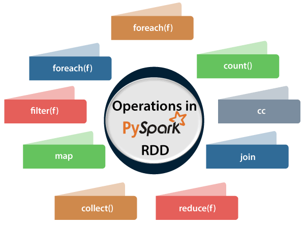
Various Operations in RDDsThe operations applied on RDDs are following: 
It returns the number of element available in RDD. Consider the following program. Output: Number of elements present in RDD : 7
This function returns the entire elements in the RDD. Output: ['python', 'java', 'hadoop', 'c', 'C++', 'spark vs hadoop', 'pyspark and spark']
The foreach(f) function returns only those elements which match the condition of the function inside foreach. Output: python java hadoop C C++ spark vs hadoop pyspark and spark
The cc operation returns a new RDD which contains the elements; those satisfy the function inside the filter. In the following example, we filter out the strings containing "spark". Output: Filtered RDD : ['spark', 'spark vs hadoop', 'pyspark', 'pyspark and spark']
It returns new RDD in a key-value pair and maps every string with a value of 1. Consider the following example: Output:
Key value pair -> [('python', 1), ('java', 1), ('hadoop', 1), ('c', 1), ('C++', 1), ('spark vs hadoop', 1), ('pyspark and spark', 1)]
It performs the specified commutative and associative binary operation in RDD. Consider the following example: Output: Adding all the elements : 15
We can check if the RDD is cached or not with cache() function. Output: Words got chached > True
It returns RDD with the matching keys with their values in paired form. We will get two different RDDs for two pair of element. Consider the following code: Output:
Join RDD -> [('hadoop', (3, 4)), ('pyspark', (1, 2))]
DataFrame from RDDPySpark provides two methods to convert a RDD to DF. These methods are given following:
When we create RDD by parallelize function, we should identify the same row element in DataFrame and wrap those element by the parentheses. The row() can accept the **kwargs argument.
We can also convert the RDD to DataFrame by using createDataFrame. Consider the following example:
Next TopicPySpark Broadcast & Accumulator
|
 For Videos Join Our Youtube Channel: Join Now
Feedback
- Send your Feedback to [email protected]
Help Others, Please Share


