Extended Euclidian Algorithm

A similar approach for determining the coefficients of Bézout's identity of two univariate polynomials and the most significant common factor of polynomials is known as the "extended Euclidean algorithm."

The extended Euclidean method is beneficial when a and b are coprime. Thus, both extended Euclidean algorithms are extensively employed in cryptography.

Description

A series of Euclidean divisions whose quotients are not utilized make up the typical Euclidean algorithm. All that is kept are the leftovers. The succeeding quotients are utilized in the extended procedure. More specifically, using a and b as input, the typical Euclidean algorithm computes a sequence of quotients (q1,.., qk) and remainders (r0,.., rk+1) such that.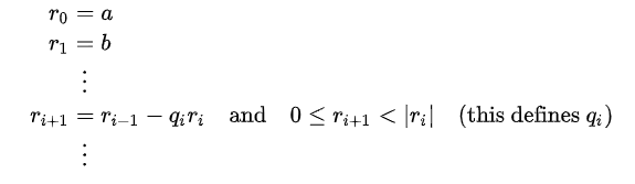

The primary characteristic of Euclidean division is that the inequalities on the right determine qi and ri+1 from ri-1 and ri in a singular way.

The greatest common divisor is the final non-zero residual, rk after the computation finishes when one reaches a remainder that is zero.

The extended Euclidean method follows a similar path but adds two more sequences.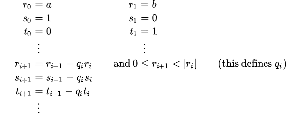

When rk+1 = 0, the calculation also comes to an end and yields

• The input variables a = r0 and b = r1 have rk as their greatest common divisor.
• Sk and tk, or gcd(a,b) = rk = ask + btk, are the Bézout coefficients.
• Given by and are the quotients of a and b by their greatest common factor.

In addition, if gcd(a,b) /= min(a,b) and a and b are both positive,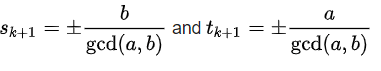

then the most significant number that is not bigger than x, where |x| signifies the integral component of x. for 0 = i = k.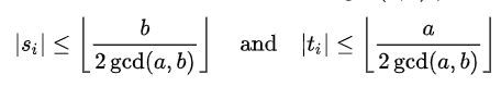

As the only pair meeting both conditions mentioned earlier, the pair of Bézout's coefficients supplied by the extended Euclidean method is the smallest pair of Bézout coefficients.

Additionally, it indicates that the technique may be implemented by a computer program utilizing numbers of a predetermined size that are greater than a and b without integer overflow.

Example

The extended Euclidean algorithm's progress using inputs 240 and 46 is depicted in the following table. The final non-zero value, 2, in the "remainder" column, is the greatest common divisor. The residual in row 6 is zero. Thus, the computation ends there. In the final two entries of the second-to-last row, there are Bézout coefficients. It is simple to confirm that 9 240 + 47 46 = 2.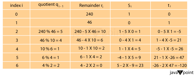

Extended Euclidean algorithm using polynomials

The first distinction is that an inequality on the degrees deg ri+1 deg ri must be used instead of the inequality 0 = ri+1 = |ri| in the Euclidean division and algorithm. Otherwise, nothing in the preceding paragraphs has changed; all that has changed is the substitution of polynomials for integers.

Another distinction is the extended Euclidean algorithm's constraint on the size of the Bézout coefficients, which is more precise in the polynomial situation and yields the following result.

The extended Euclidean method creates the specific pair of polynomials (s, t) such that as + bt = gcd(a,b) if a and b are two non-zero polynomials.

There are several approaches to establish the most significant common factor.

It is typical in mathematics to demand that the most significant common divisor be mononomial. Divide each output element by the leading coefficient of rk to obtain this. This enables one to obtain 1 on the right-hand side of Bézout's inequality if a and b are coprime. Otherwise, any non-zero constant might be obtained. Since the polynomials in computer algebra frequently contain integer coefficients, normalizing the greatest common divisor in this method adds too many fractions to be practical.

Divide each output element by the leading coefficient of rk to obtain this. This enables one to obtain 1 on the right-hand side of Bézout's inequality if a and b are coprime. Otherwise, any non-zero constant might be obtained. Since the polynomials in computer algebra frequently contain integer coefficients, normalizing the greatest common divisor in this method adds too many fractions to be practical.

The normalization also yields a maximum common factor of one of the input polynomials coprime.

Thirdly, we extend the subresultant pseudo-remainder sequences method similarly to the extended Euclidean algorithm from the original subresultant pseudo-remainder sequences algorithm. Starting with integer coefficients enables all computed polynomials to have integer coefficients. Furthermore, each computed remainder, ri, is a subresultant of a polynomial. The equation has no denominator for this interpretation of Bézout's identity. By dividing everything by the outcome, the conventional Bézout's identity is obtained, which has a different common denominator for the rational numbers that occur in it.

Starting with integer coefficients enables all computed polynomials to have integer coefficients. Furthermore, each computed remainder, ri, is a subresultant of a polynomial. The equation has no denominator for this interpretation of Bézout's identity. By dividing everything by the outcome, the conventional Bézout's identity is obtained, which has a different common denominator for the rational numbers that occur in it.

Pseudocode

First, it should be noted that the indexed variables' two most recent values are required at each stage when implementing the above-described algorithm. Therefore, each indexed variable must be replaced by simply two variables to conserve memory.

The following algorithm, as well as the others in this article, employs parallel assignments for simplicity. Auxiliary variables must be used to emulate concurrent assignments in programming languages without this functionality.

For example, the first one,

is equivalent to

and similarly for the other parallel assignments. This leads to the following code:

The result may be wrong when dividing a and b by their GCD. This is simple to fix after the calculation, but it has yet to be done here for code simplicity. Like the previous example, all output signs must be altered if either an or b is zero and the other is negative. In this case, the output's greatest common divisor is also harmful.

In Bézout's identity, axe + by = gcd(a,b), y may be solved if a, b, x, and gcd(a,b) are known. The Bézout coefficient x may be obtained by computing only the sk sequence, which is an improvement to the following algorithm:

This suggests that the "optimization" substitutes a series of little integer multiplications and divisions with a single operation that takes more time to compute than the operations it replaces altogether. The three output lines of the previous pseudocode can be replaced with the following lines to create this canonical reduced version.

Because s and t are two coprime numbers, + bt = 0, and so on, the proof of this procedure depends on this fact. Moving the negative sign to indicate a positive denominator is all necessary to obtain the simplified canonical version.

If b divides equally, the algorithm does one iteration, resulting in s = 1.

Utilizing modular frameworks to compute multiplicative inverses.

Flexible integers

If n is a positive integer, the set of remainders from Euclidean division by n is known as the ring Z/nZ. The addition and multiplication operations involve dividing the sum of the addition and multiplication of integers by n. If an element an of Z/nZ is coprime to n, it has a multiplicative inverse (i.e., it is a unit) otherwise.

The multiplicative inverse of a modulo n is thus t, or more precisely, the residue of the division of t by n.

To apply the extended Euclidean method to this issue, it should be noted that the computation of the n-th Bézout coefficient is not required. Additionally, one may exploit the fact that the integer t produced by the procedure fulfills |t| n to obtain a positive and less than n result. In other words, if t 0, n must be added at the end. This generates the pseudocode, where n is an integer greater than 1.

The extended Euclidean algorithm is the primary method for computing multiplicative inverses in extensions of simple algebraic fields. Finite fields of non-prime order are frequently employed in cryptography and coding theory.

The procedure for computing the modular multiplicative inverse is similar to before. There are two significant variations: first, the last line is not required since the supplied Bézout coefficient always has a degree lower than d. Second, any non-zero members of K may serve as the greatest common divisor when the input polynomials are coprime; as a result, this Bézout coefficient (a polynomial often of positive degree) must be multiplied by the inverse of this element of K. The polynomial p and the polynomial an are polynomials in the following pseudocode.

There are two significant variations: first, the last line is not required since the supplied Bézout coefficient always has a degree lower than d. Second, any non-zero members of K may serve as the greatest common divisor when the input polynomials are coprime; as a result, this Bézout coefficient (a polynomial often of positive degree) must be multiplied by the inverse of this element of K. The polynomial p and the polynomial an are polynomials in the following pseudocode.

Example

For instance, if a = x6 + x4 + x + 1 is, the element whose inverse is needed and p = x8 + x4 + x3 + x + 1 is the polynomial used to create the finite field GF(28), then using the technique yields the calculation shown in the following table. For every element z in the field, z + z = 0 exists in fields of order 2n. The modification in the last line of the pseudocode is unnecessary because 1 is the sole non-zero member in GF(2).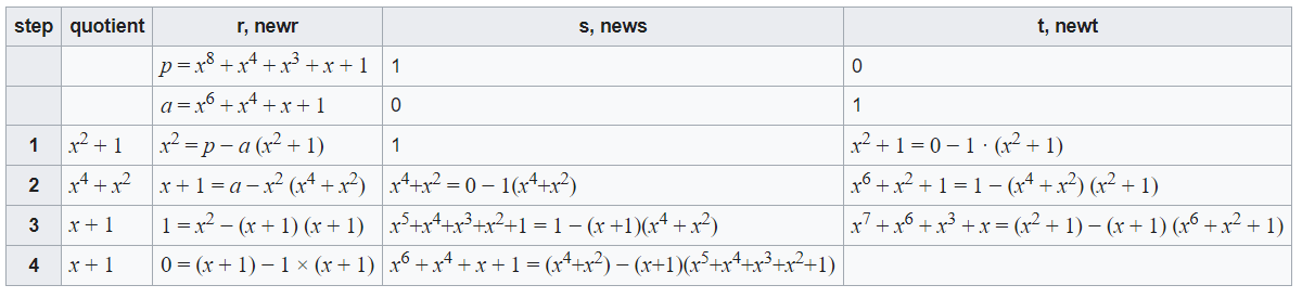

By multiplying the two components together and then multiplying the residual by p, it is proven that the inverse is x7 + x6 + x3 + x.

More than two integers are involved.

Iteratively handling cases with more than two numbers is possible. We begin by demonstrating that gcd(a, b, c) = gcd(gcd(a, b), c)). Let d = gcd(a, b, c) demonstrate this. D is a divisor of a and b according to the gcd definition. Therefore, for some k, gcd(a, b) = kd. Similar to how d divides c, c equals jd for some j. Suppose u = gcd(k,j). According to our method of constructing you, ud|a, b, and c, but since d is u's largest divisor, you is a unit. Because ud = gcd(gcd(a, b), c)), the conclusion is established.

Iteratively handling cases with more than two numbers is possible. We begin by demonstrating that gcd(a, b, c) = gcd(gcd(a, b), c)). Let d = gcd(a, b, c) demonstrate this. D is a divisor of a and b according to the gcd definition. Therefore, for some k, gcd(a, b) = kd. Similar to how d divides c, c equals jd for some j. Suppose u = gcd(k,j). According to our method of constructing you, ud|a, b, and c, but since d is u's largest divisor, you is a unit. Because ud = gcd(gcd(a, b), c)), the conclusion is established.

More than two integers are involved.

Iteratively handling cases with more than two numbers is possible. We begin by demonstrating that gcd(a, b, c) = gcd(gcd(a, b), c)). Let d = gcd(a, b, c) demonstrate this. D is a divisor of a and b according to the gcd definition. Therefore, for some k, gcd(a, b) = kd. Similar to how d divides c, c equals jd for some j. Suppose u = gcd(k,j). According to our method of constructing u, ud|a, b, and c, but since d is u's largest divisor, u is a unit. Because ud = gcd(gcd(a, b), c)), the conclusion is established.