Sorting Algorithms: Slowest to Fastest

In the following tutorial, we will discuss the different sorting algorithms and compare them on the basis of their complexities.

So, let's get started.

What is a Sorting Algorithm?

The sorting Algorithm is a set of instructions that accepts an array or list as an input and arranges the data elements into a specific order.

Sorts are most commonly in numerical or a form of alphabetical (or lexicographical) format, and the sorting order can either be ascending (0 - 9, A - Z) or descending (9 - 0, Z - A).

Understanding the Importance of Sorting Algorithms

Sorting Algorithms serve a significant role in Computer Science, as they can often reduce the complexity of a problem. These algorithms have direct applications in searching algorithms, database management algorithms, data structure algorithms, divide and conquer methods, and many more.

Some of the best examples of real-world implementation of the sorting algorithms are:

The bubble Sort Algorithm is generally used in programming TV in order to sort channels on the basis of audience viewing time.
Databases utilize an external Merge Sort Algorithm in order to sort the set of data that is too large to be loaded completely into the memory.
Sports scores are quickly organized using the Quick Sort Algorithm in real-time.
Apart from the above, many other real-life examples of sorting algorithms exist.

Understanding the Types of Sorting in Data Structures

The sorting Technique in Data Structures is divided into types:

Comparison-based Sorting: In Comparison-based sorting techniques, a comparator is defined in order to compare the data elements or items of a data sample. This comparator states the ordering of elements. Some Examples of Comparison-based sorting are Bubble Sort and Merge Sort.
Counting-based Sorting: In Counting-based sorting techniques, no comparison is involved between the data elements of a data sample; however, it works on calculated assumptions during execution. Some examples of Counting-based sorting are Counting Sort and Radix Sort.
In-Place and Not-in-Place Sorting Techniques: In-Place sorting techniques in data structures are used to modify the ordering of array elements within the original array.

At the same time, the Not-in-Place sorting techniques make use of an auxiliary data structure in order to sort the original array. Some examples of In-Place sorting techniques are Bubble Sort and Selection Sort. Some examples of Not-in-Place sorting algorithms are Merge Sort and Quick Sort.

Some Common Sorting Algorithms

The following is the list of some commonly used Sorting Algorithms:

Bubble Sort
Selection Sort
Insertion Sort
Quick Sort
Merge Sort
Counting Sort
Radix Sort
Bucket Sort
Comb Sort
Shell Sort

Let us examine the above sorting algorithms with their time and space complexities to determine the fastest Sorting Algorithm.

Bubble Sort

Bubble Sort is the simplest sorting algorithm. The fundamental concept behind bubble sorting is that it repeatedly swaps adjacent data elements if they are not in the desired order.

Suppose a given array of data elements has to be sorted in ascending order. In that case, bubble sort will start by comparing the first data element of the array with the second one and immediately swap them if it turns out to be a larger value than the second element, and then move on to comparing the second and third data elements, and so on.

Let us understand the intuitive approach behind the bubble sort using an example:

Example:

Suppose we are given an array of five different data elements arranged unsorted.

Given Array : (5, 3, 4, 2, 1)

We will now use the bubble sort to arrange these data elements of the array in ascending order.

First Iteration:

(5, 3, 4, 2, 1) -> (3, 5, 4, 2, 1)

The bubble sort compares the first two data elements and swaps since 5 is greater than 3 (5 > 3).

(3, 5, 4, 2, 1) -> (3, 4, 5, 2, 1), swaps since 5 is greater than 4 (5 > 4)
(3, 4, 5, 2, 1) -> (3, 4, 2, 5, 1), swaps since 5 is greater than 2 (5 > 2)
(3, 5, 2, 5, 1) -> (3, 4, 2, 1, 5), swaps since 5 is greater than 1 (5 > 1)

Second Iteration:

(3, 4, 2, 1, 5) -> (3, 2, 4, 1, 5), swaps since 4 is greater than 2 (4 > 2)
(3, 2, 4, 1, 5) -> (3, 2, 1, 4, 5), swaps since 4 is greater than 1 (4 > 1)

Third Iteration:

(3, 2, 1, 4, 5) -> (2, 3, 1, 4, 5), swaps since 3 is greater than 2 (3 > 2)
(2, 3, 1, 4, 5) -> (2, 1, 3, 4, 5), swaps since 3 is greater than 1 (3 > 1)

Fourth Iteration:

(2, 1, 3, 4, 5) -> (1, 2, 3, 4, 5), swaps since 2 is greater than 1 (2 > 1)
The algorithm requires one complete pass without any swap to check if it is sorted.
(1, 2, 3, 4, 5) -> (1, 2, 3, 4, 5)
Hence, we have successfully sorted our array in ascending order.

Now that we have understood the intuitive concept behind the bubble sort, it is time for us to consider its standard implementation in C++ Programming Language.

Implementation of Bubble Sort in C++

// including the required header file
# include <bits/stdc++.h>

// using the standard namespace
using namespace std;

// defining a function to perform Bubble Sort
void BubbleSort(int arr[], int size){
    
    // defining some iterables
    int i, j;

    // using a nested for-loop
    for (i = 0; i < size - 1; i++)
        for (j = 0; j < size - i - 1; j++)
            // comparing the values of adjacent elements and swaping them if the first one is greater than the other 
            if (arr[j] > arr[j + 1])
                swap(arr[j], arr[j + 1]);
}

// main function
int main(){
    // defining and initializing an array
    int arr[] = {5, 3, 4, 2, 1};

    // calculating the size of array
    int size = sizeof(arr) / sizeof(arr[0]);

    // printing the unsorted array for the users
    cout << "Unsorted Array : \n";
    for (int i = 0; i < size; i++)
        cout << arr[i] << " ";
    cout << endl;

    // calling the BubbleSort() function to sort the given array in ascending order
    BubbleSort(arr, size);

    // printing the sorted array for the users
    cout << "Sorted Array : \n";
    for (int i = 0; i < size; i++)
        cout << arr[i] << " ";
    cout << endl;

    return 0;
}

Output:

Unsorted Array : 
5 3 4 2 1 
Sorted Array : 
1 2 3 4 5

Explanation:

In the above code snippet, we included the 'bits/stdc++.h' header file and used the standard namespace. We have then defined the void function as BubbleSort(), which accepts two arguments - array name and its size. Inside this function, we have defined two iterables, i and j. We have used the nested for-loop to iterate through each element of the array, compare the current element's value with the next element, and swap their positions if it is larger.

Now inside the main function, we have defined and initialized an unsorted array as arr. We then calculated its size. We have also printed the elements of the unsorted array for the users. We have then called the BubbleSort() function by passing the array name, i.e., arr, and its size. At last, we have printed the sorted array elements for the users.

As a result, the given array, i.e., (5, 3, 4, 2, 1), is sorted into ascending order as (1, 2, 3, 4, 5).

Performance Analysis of Bubble Sort

Let us now observe the Time complexity of Bubble Sort in the best case, average case, and worst case. We will also observe the Space complexity of Bubble Sort.

Time Complexity:

Worst Case: O(n²)
Average Case: Θ(n²)
Best Case: Ω(n)

Auxiliary Space Complexity: O(1)

Some Applications of Bubble Sort

The following are some applications of Bubble Sort:

Bubble Sort is used to introduce the fundamental concepts of a sorting algorithm to Computer Science students.
Bubble Sort is quite famous in computer graphics for detecting a small error (for example, swapping only two data elements) in almost-sorted arrays.

Selection Sort

Selection Sort is a sorting algorithm where the given array is divided into two sub-arrays -

The first sub-array will consist of the sorted part of the list.
The second sub-array will consist of the unsorted part of the list.

Primarily, the sorted segment remains empty whereas the unsorted segment contains the complete list. In each iteration, we will fetch the smallest data element from the unsorted sub-array and push it to the end of the sorted sub-array. Thus, we can successfully construct our sorted array.

Let us understand the intuitive approach behind the selection sort using an example:

Example:

Suppose we are given an array of five different data elements arranged unsorted.

Given Array : (26, 23, 28, 16, 18)

We will now use the selection sort to arrange these data elements of the array in ascending order.

For i = 0, we will select the smallest element of the array, i.e., 16, and move it to the beginning of the unsorted array at i = 0 preserving the relative order of the remaining data elements.

Therefore, we will get the following array:

(16, 26, 23, 28, 18)

Similarly, for i = 1, we will again select the next smallest element of the array, i.e., 18, and move it to the beginning of the unsorted array at i = 1 preserving the relative order of the remaining data elements.

Therefore, we will now get the following array:

(16, 18, 26, 23, 28)

Similarly, for i = 2, we will again select the next smallest element of the array, i.e., 23, and move it to the beginning of the unsorted array at i = 2 preserving the relative order of the remaining data elements.

Therefore, we will now get the following array:

(16, 18, 23, 26, 28)

Similarly, for i = 3, we will again select the next smallest element of the array, i.e., 26, and move it to the beginning of the unsorted array at i = 3 preserving the relative order of the remaining data elements.

Therefore, we will now get the following array:

(16, 18, 23, 26, 28)

Similarly, for i = 4, we will again select the next smallest element of the array, i.e., 28, and move it to the beginning of the unsorted array at i = 4.

Hence, the final sorted array will be:

(16, 18, 23, 26, 28)

Now that we have understood the intuitive concept behind the selection sort, it is time for us to consider its standard implementation in C++ Programming Language.

Implementation of Selection Sort in C++

// including the required header file
# include <bits/stdc++.h>

// using the standard namespace
using namespace std;

// defining a function to perform Selection Sort
void SelectionSort(int arr[], int size){
    
    // defining iterables and variables
    int i, j, curr;
    
    // using the nested for-loop
    for (i = 0; i < size - 1; i++){
        // initializing the curr variable as i
        curr = i;
        for (j = i + 1; j < size; j++)
            // if array's element at index j is lower than element at the curr variable, then set the curr to j 
            if (arr[j] < arr[curr])
                curr = j;
        // calling the swap() function to swap the lowest value with the current index i curr
        swap(arr[curr], arr[i]);
    }
}

// main function
int main(){
    // defining and initializing an array
    int arr[] = {25, 23, 28, 16, 18};
    
    // calculating the size of array
    int size = sizeof(arr)/sizeof(arr[0]);

    // printing the unsorted array for the users
    cout << "Unsorted Array : \n";
    for (int i = 0; i < size; i++)
        cout << arr[i] << " ";
    cout << endl;

    // calling the SelectionSort() function to sort the given array in ascending order    
    SelectionSort(arr, size);

    // printing the sorted array for the users
    cout << "Sorted Array : \n";
    for (int i = 0; i < size; i++)
        cout << arr[i] << " ";
    cout << endl;

    return 0;
}

Output:

Unsorted Array : 
25 23 28 16 18
Sorted Array :
16 18 23 25 28

Explanation:

In the above code snippet, we included the 'bits/stdc++.h' header file and used the standard namespace. We have then defined the void function as SelectionSort(), which accepts two arguments - array name and its size. Inside this function, we have defined two iterables, i and j and a variable as curr. We have used the nested for-loop to iterate through each element of the array. Inside the first for-loop, we have initialized the curr variable as the current value of index i. Inside the second for-loop, we have compared the element value at index j is less than element at position curr and called the swap() function to swap their positions if it is larger.

Now inside the main function, we have defined and initialized an unsorted array as arr. We then calculated its size. We have also printed the elements of the unsorted array for the users. We have then called the SelectionSort() function by passing the array name, i.e., arr, and its size. At last, we have printed the sorted array elements for the users.

As a result, the given array, i.e., (25, 23, 28, 16, 18), is sorted into ascending order as (16, 18, 23, 25, 28).

Performance Analysis of Selection Sort

Let us now observe the Time complexity of Selection Sort in the best case, average case, and worst case. We will also observe the Space complexity of Selection Sort.

Time Complexity:

Worst Case: O(n²)
Average Case: Θ(n²)
Best Case: Ω(n²)

Auxiliary Space Complexity: O(1)

Some Applications of Selection Sort

The following are some applications of Selection Sort:

Selection Sort is used for the small size of the data list since the time complexity of this sorting algorithm is O(n²), making it incompetent for a large list.
Selection Sort is also utilized for limited memory space because it makes the minimum possible number of swaps throughout the sorting process.

Insertion Sort

Insertion Sort is a sorting algorithm in which the given array is divided into a sorted and an unsorted segment. In each iteration, we have to find the optimal position of the data element to be inserted in the sorted subsequence and then insert it while shifting the remaining data elements to the right side.

Let us understand the intuitive approach behind the insertion sort using an example:

Example:

Suppose we are given an array of five different data elements arranged unsorted.

Given Array : (26, 23, 28, 16, 18)

We will now use the insertion sort to arrange these data elements of the array in ascending order.

For i = 1, since 23 is a smaller value than 26, we will move 25 to the right and insert the data element with 23 before 25.

Therefore, we will get the following array:

(23, 26, 28, 16, 18)

For i = 2, since all the elements in A[0, …, i-1] are smaller than 27, it will remain as it is in its position.

Therefore, our array will remain unchanged:

(23, 26, 28, 16, 18)

For i = 3, we will move the data element with value 16 to the beginning, shifting the rest of the data elements from 23 to 28 to one position to the right.

Therefore, we will get the following array:

(16, 23, 26, 28, 18)

For i = 4, we will move the data element having value 18 after 16, and data elements from 23 to 28 will be shifted one position to the right.

Hence, the final sorted array will be:

(16, 18, 23, 26, 28)

Now that we have understood the intuitive concept behind the insertion sort, it is time for us to consider its standard implementation in C++ Programming Language.

Implementation of Insertion Sort in C++

// including the required header file
# include <bits/stdc++.h>

// using the standard namespace
using namespace std;

// defining a function to perform Insertion Sort
void InsertionSort(int arr[], int size){

    // defining some iterables and variables
    int i, temp, j;

    // using the for-loop
    for (i = 1; i < size; i++){
        // initializing the temp variable as value at index i from array
        temp = arr[i];
        // initializing another iterable value
        j = i - 1;
        // using the while loop for j >= 0 and arr[j] > temp
        while (j >= 0 && arr[j] > temp){
            // swapping the elements
            arr[j + 1] = arr[j];
            j = j - 1;
        }
        arr[j + 1] = temp;
    }
}

// main function
int main(){
    // defining and initializing an array
    int arr[] = {25, 23, 28, 16, 18};

    // calculating the size of array
    int size = sizeof(arr) / sizeof(arr[0]);

    // printing the unsorted array for the users
    cout << "Unsorted Array : \n";
    for (int i = 0; i < size; i++)
        cout << arr[i] << " ";
    cout << endl;

    // calling the InsertionSort() function to sort the given array in ascending order    
    InsertionSort(arr, size);

    // printing the sorted array for the users
    cout << "Sorted Array : \n";
    for (int i = 0; i < size; i++)
        cout << arr[i] << " ";
    cout << endl;

    return 0;
}

Output:

Unsorted Array : 
25 23 28 16 18
Sorted Array :
16 18 23 25 28

Explanation:

We included the 'bits/stdc++.h' header file in the above code snippet and used the standard namespace. We have then defined the void function as InsertionSort(), which accepts two arguments - array name and its size. Inside this function, we have defined two iterables, i and j, and a variable as the temp. We have used the for-loop to iterate through each element of the array. Inside this, we have initialized the temp variable as the value at arr[i] and iterable j as the value preceding that of i. We then used the while loop to compare the element value at index j and temp and swap their positions if larger.

Now inside the main function, we have defined and initialized an unsorted array as arr. We then calculated its size. We have also printed the elements of the unsorted array for the users. We have then called the InsertionSort() function by passing the array name, i.e., arr, and its size. At last, we have printed the sorted array elements for the users.

As a result, the given array, i.e., (25, 23, 28, 16, 18), is sorted into ascending order as (16, 18, 23, 25, 28).

Performance Analysis of Insertion Sort

Let us now observe the Time complexity of Insertion Sort in the best case, average case, and worst case. We will also observe the Space complexity of Insertion Sort.

Time Complexity:

Worst Case: O(n²)
Average Case: Θ(n²)
Best Case: Ω(n)

Auxiliary Space Complexity: O(1)

Some Applications of Insertion Sort

The following are some applications of Insertion Sort:

Insertion Sort is a stable sorting algorithm that works quickly when the list is almost sorted.
Insertion Sort is very effective and efficient when sorting a small data list (for example, 35 data elements).

Quick Sort

Quick Sort is a sorting algorithm that works on the divide and conquer approach. The instinctive concept behind this sorting technique is it chooses a data element as the pivot from a given array of data elements and then partitions the array around that pivot data element. Consequently, it calls itself recursively portioning the two subarrays afterward.

Let us understand the intuitive approach behind the quick sort using an example:

Example: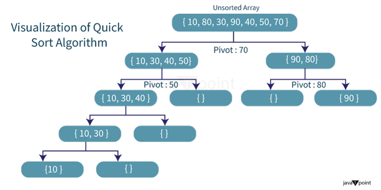

The logical steps included in the Quick Sort algorithm are as shown below:

Pivot Selection: We will first select a data element as the pivot (in this case, we have chosen the last data element as the pivot).
Partitioning: We will then partition the array in a manner such that all the data elements less than the pivot are in the left sub-array, whereas the data elements strictly greater than the pivot element are stored in the right sub-array.
The Recursive Call to Quicksort: We will invoke the Quicksort function again for the two sub-arrays created above and repeat the process until we get the final sorted array.

Now that we have understood the intuitive concept behind the quick sort, it is time for us to consider its standard implementation in C++ Programming Language.

Implementation of Quick Sort in C++

// including the required header file
# include <bits/stdc++.h>

// using the standard namespace
using namespace std;

// defining a function to partition_array the array around the pivot_element
int partition_array(int arr[], int start, int end){
    // defining and initializing the pivot element
    int pivot_element = arr[end];
    // defining and initializing an iterable
    int i = (start - 1);
    // using the for-loop to iterate through the array and swap the elements for sorting
    for (int j = start; j <= end - 1; j++){
        if (arr[j] < pivot_element){
            i++; swap(arr[i], arr[j]);
        }
    }
    swap(arr[i + 1], arr[end]);
    return (i + 1);
}
 
/*
arr[] --> array to be sorted,
start --> Starting index,
end --> Ending index
*/

// defining a function to perform Quick Sort
void QuickSort(int arr[], int start, int end){
    if (start < end){
        // middle is partitioning index, arr[p] is now at right place
        int middle = partition_array(arr, start, end);
        // sorting data elements seperately before partition and after partition
        QuickSort(arr, start, middle - 1);
        QuickSort(arr, middle + 1, end);
    }
}

// main function
int main(){
    // defining and initializing an array
    int arr[] = {25, 23, 28, 16, 18};

    // calculating the size of array
    int size = sizeof(arr) / sizeof(arr[0]);

    // printing the unsorted array for the users
    cout << "Unsorted Array : \n";
    for (int i = 0; i < size; i++)
        cout << arr[i] << " ";
    cout << endl;

    // calling the QuickSort() function to sort the given array in ascending order    
    QuickSort(arr, 0, size - 1);

    // printing the sorted array for the users
    cout << "Sorted Array : \n";
    for (int i = 0; i < size; i++)
        cout << arr[i] << " ";
    cout << endl;

    return 0;
}

Output:

Unsorted Array : 
25 23 28 16 18
Sorted Array :
16 18 23 25 28

Explanation:

We included the 'bits/stdc++.h' header file in the above code snippet and used the standard namespace. We have then defined the function as partition_array() to partition the array around the pivot element. This function accepts three arguments - array name, start point, and end point. Inside this function, we have initialized a value of the pivot element and defined an iterable for iteration. We then used the for-loop to iterate through the elements and swap the elements to sort the array. We have then defined the void function as QuickSort(), which accepts three arguments - array name, start point, and end point. Inside this function, we have compared if the starting point is lower than the ending point and called the partition_array() function. We have then recursively called the QuickSort() function.

Now inside the main function, we have defined and initialized an unsorted array as arr. We then calculated its size. We have also printed the elements of the unsorted array for the users. We then called the QuickSort() function by passing the array name and starting and ending points. At last, we have printed the sorted array elements for the users.

As a result, the given array, i.e., (25, 23, 28, 16, 18), is sorted into ascending order as (16, 18, 23, 25, 28).

Performance Analysis of Quick Sort

Let us now observe the Time complexity of Quick Sort in the best case, average case, and worst case. We will also observe the Space complexity of Quick Sort.

Time Complexity:

Worst Case: O(n²)
Average Case: Θ(n * log n)
Best Case: Ω(n * log n)

Auxiliary Space Complexity: O(log n)

Some Applications of Quick Sort

The following are some applications of Quick Sort:

Quick Sort is probably more effective for datasets that fit in memory.
Quick Sort is suitable for arrays since it is an in-place sorting algorithm that does not require any extra storage.

Merge Sort

Merge Sort is another sorting algorithm that works on the divide and conquer approach. In each iteration, merge sort divides the input array into two equal sub-arrays, calls itself recursively for the two sub-arrays, and finally merges the two sorted halves.

Let us understand the intuitive approach behind the merge sort using an example: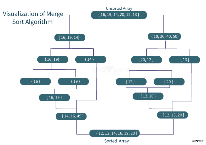

Now that we have understood the intuitive concept behind the merge sort, it is time for us to consider its standard implementation in C++ Programming Language.

Implementation of Merge Sort in C++

// including the required header file
# include <bits/stdc++.h>

// using the standard namespace
using namespace std;

// defining a function to merge the sub-arrays
void merge_subarray(long arr[], long start, long middle, long end){
    // defining some variables
    long num1 = middle - start + 1;
    long num2 = end - middle;
    
    // defining some arrays
    long Left[num1], Right[num2];
    // inserting elements to the arrays using the for-loops
    for (long i = 0; i < num1; i++)
        Left[i] = arr[start + i];
    for (long j = 0; j < num2; j++)
        Right[j] = arr[middle + 1 + j];
    
    // defining some iterables
    long i = 0, j = 0;
    long k = start;

    // using the while loop and swapping the elements to sort the array 
    while (i < num1 and j < num2) {
        if (Left[i] <= Right[j]) {
            arr[k] = Left[i]; i++;
        }
        else {
            arr[k] = Right[j]; j++;
        }
        k++;
    }
    while (i < num1) {
        arr[k] = Left[i]; i++; k++;
    }
    while (j < num2) {
        arr[k] = Right[j]; j++; k++;
    }
}

// defining a function to perform Merge Sort
void MergeSort(long arr[], long start, long end){
    // returning, if the starting point is greater than and equal to the ending point
    if(start >= end)
        return;
    // defining and initializing a variable
    long middle = start + (end - start) / 2;

    // recursively calling the MergeSort() function
    MergeSort(arr, start, middle);
    MergeSort(arr, middle + 1, end);

    // calling the merge_subarray() function
    merge_subarray(arr, start, middle, end);
}

// main function
int main(){
    // defining and initializing an array
    long arr[] = {25, 23, 28, 16, 18};

    // calculating the size of array
    long size = sizeof(arr) / sizeof(arr[0]);

    // printing the unsorted array for the users
    cout << "Unsorted Array : \n";
    for (int i = 0; i < size; i++)
        cout << arr[i] << " ";
    cout << endl;

    // calling the MergeSort() function to sort the given array in ascending order    
    MergeSort(arr, 0, size - 1);

    // printing the sorted array for the users
    cout << "Sorted Array : \n";
    for (int i = 0; i < size; i++)
        cout << arr[i] << " ";
    cout << endl;

    return 0;
}

Output:

Unsorted Array : 
25 23 28 16 18
Sorted Array :
16 18 23 25 28

Explanation:

We included the 'bits/stdc++.h' header file in the above code snippet and used the standard namespace. We have then defined the function as merge_subarray() that accepts multiple arguments like an array name, starting point, middle point, and ending point. Inside this function, we have defined some variables along with some arrays. We have then inserted the elements into these arrays using the for-loop. We have then defined and initialized some iterables and used the while loop to sort the sub-arrays by swapping their elements. We have then defined another function as MergeSort() that accepts three parameters - array name, starting point, and ending point. Inside this function,

we have used the if conditional statement to check whether the starting point is greater than or equal to the ending point and added a return statement to break the loop. We have then defined and initialized a variable as middle and recursively called MergeSort() function to sort the array. We have then called the merge_subarray() function.

Now inside the main function, we have defined and initialized an unsorted array as arr. We then calculated its size. We have also printed the elements of the unsorted array for the users. We then called the MergeSort() function by passing the array name and starting and ending points. At last, we have printed the sorted array elements for the users.

As a result, the given array, i.e., (25, 23, 28, 16, 18), is sorted into ascending order as (16, 18, 23, 25, 28).

Performance Analysis of Merge Sort

Let us now observe the Time complexity of Merge Sort in the best case, average case, and worst case. We will also observe the Space complexity of Merge Sort.

Time Complexity:

Worst Case: O(n * log n)
Average Case: Θ(n * log n)
Best Case: O(n * log n)

Auxiliary Space Complexity: O(n)

Some Applications of Merge Sort

The following are some applications of Merge Sort:

Merge Sort is fast in the case of data structures like linked lists.
Merge Sort is extensively utilized for external sorting where random access can be pretty expensive compared to sequential access.

Counting Sort

Counting Sort is a fascinating sorting algorithm primarily focusing on the frequency of unique data elements between a particular range (something along the lines of hashing).

This sorting algorithm works by counting the number of data elements having distinct key values and then building a sorted array after estimating the position of each unique data element in the unsorted sequence.

Counting Sort stands apart from the algorithms we discussed earlier as it involves zero comparisons between the input data elements.

Let us understand the intuitive approach behind the counting sort using an example:

Example:

For simplicity, suppose we are given an unsorted array of data elements ranging from 0 to 3.

Given Array : (1, 0, 3, 1, 3, 1)
First of all, we will build a frequency array in order to store the count of each unique element.

Index	0	1	2	3
Counter	1	3	0	2

We will now modify the counter array to form a prefix sum array as shown below:

Index	0	1	2	3
Counter	1	4	4	6

The modified counter array indicates the position of each object in the output sequence.
Output each object from the input sequence followed by decreasing its count by 1. The following array is built by shifting each data element from 1 place to the right.

Index	0	1	2	3
Counter	0	1	4	4

Now process the input data : 1, 0, 3, 1, 3, 1

The position of 2 is 4 as per the final array (step 3). Thus, we put data 2 at index 4 in the output sequence simultaneously decreasing its count by 1 to place next data 2 at an index 3 smaller than the current index.
Extending this approach for the complete input array, we will get the sorted sequence as shown below:

Final Array : (0, 1, 1, 1, 3, 3)

Now that we have understood the intuitive concept behind the counting sort, it is time for us to consider its standard implementation in C++ Programming Language.

Implementation of Counting Sort in C++

// including the required header file
# include <bits/stdc++.h>

// using the standard namespace
using namespace std;

// defining the function to get the maximum value from the array
long getMaximum(long arr[], long size) {
    // defining and initializing an initial maximum value from the array
    long maximum = arr[1];
    // using the for-loop to iterate through the array
    for(long i = 2; i <= size; i++) {
        // updating the value in the maximum variable with the maximum value from the array
        if(arr[i] > maximum)
            maximum = arr[i];
    }
    // returning the final maximum value
    return maximum;
}

// defining the function to perform Counting Sort
void CountingSort(long *arr, long size) {
    // defining an array for output
    long output_array[size + 1];
    
    // calling the getMaximum() function and storing the returned value in a variable
    long maximum = getMaximum(arr, size);
    
    // defining an array to store count
    long counter[maximum + 1];
    
    // using the for-loop to set the initial values of the elements of the counter array to 0 
    for(long i = 0; i <= maximum; i++)
        counter[i] = 0;

    // using the for-loop to update the values in the counter array for the given array
    for(long i = 1; i <= size; i++)
        counter[arr[i]]++;
    
    // using the for-loop to modify the counter array to form a prefix sum array
    for(long i = 1; i <= maximum; i++)
        counter[i] += counter[i - 1];
    
    // using the for-loop to generate the output from the input sequence followed by decreasing its count by 1    
    for(long i = size; i >= 1; i--) {
        output_array[counter[arr[i]]] = arr[i];
        counter[arr[i]] -= 1;
    }

    // using the for-loop to update the values in the original array using output array
    for(long i = 1; i <= size; i++) {
        arr[i] = output_array[i];
    }
}

// main function
int main(){
    // defining and initializing an array
    long arr[] = {0, 1, 0, 3, 1, 3, 1};

    // calculating the size of array
    long size = sizeof(arr) / sizeof(arr[0]);

    // printing the unsorted array for the users
    cout << "Unsorted Array : \n";
    for (int i = 1; i < size; i++)
        cout << arr[i] << " ";
    cout << endl;

    // calling the CountingSort() function to sort the given array in ascending order    
    CountingSort(arr, size - 1);

    // printing the sorted array for the users
    cout << "Sorted Array : \n";
    for (int i = 1; i < size; i++)
        cout << arr[i] << " ";
    cout << endl;

    return 0;
}

Output:

Unsorted Array : 
1 0 3 1 3 1
Sorted Array :
0 1 1 1 3 3

Explanation:

We included the 'bits/stdc++.h' header file in the above code snippet and used the standard namespace. We have then defined the function as getMaximum() that accepts two parameters as the array name and its size in order to retrieve the maximum value from the array. Inside this function, we have first initialized a variable with an initial maximum value. We then iterated through the array, updated the variable value with the final maximum value, and returned it. We have then defined another function as CountingSort(), that accepts two parameters as the array name and its size. Inside this function, we have defined an array to store the output, called the getMaximum() function, and a counter array. We have then used the for-loop to set the initial values of the elements in the counter array to 0. We have again used the for-loop to update the values in the counter array for the given array. We then iterated through the counter array again using the for-loop, modifying its value to form a prefix sum array. Again, we used the for-loop to generate the output from the input sequence, then decreased its count by 1. At last, we have used the for-loop to iterate through the data elements of the array and update their values in respect of the output array.

Now inside the main function, we have defined and initialized an unsorted array as arr. We then calculated its size. We have also printed the elements of the unsorted array for the users. We then called the CountingSort() function by passing the array name and starting and ending points. At last, we have printed the sorted array elements for the users.

As a result, the given array, i.e., (1, 0, 3, 1, 3, 1), is sorted into ascending order as (0, 1, 1, 1, 3, 3).

Performance Analysis of Counting Sort

Let us now observe the Time complexity of Counting Sort in the best case, average case, and worst case. We will also observe the Space complexity of Counting Sort.

Time Complexity:

Worst Case: O(n + k)
Average Case: Θ(n + k)
Best Case: Ω(n + k)

Auxiliary Space Complexity: O(k), where k is the count of unique elements in the array.

Some Applications of Counting Sort

The following are some applications of Counting Sort:

Counting Sort is a pretty efficient sorting algorithm for sorting countable objects (like bounded integers).
Counting Sort is also utilized when sorting is done in linear complexity.

Radix Sort

As we have already discussed, Counting Sort stands apart because it is not a comparison-based sorting algorithm similar to Merge Sort or Bubble Sort. Thus, we can reduce its time complexity to linear time.

However, this sorting technique fails when the data elements of the input array range from 1 to n², which results in an increase of its time complexity to O(n²).

The fundamental concept behind radix sorting is to extend the functionality of counting sort to achieve a better time complexity when the data elements of the input array range from 1 to n².

Let us understand this sorting algorithm in brief:

Algorithm:

For each digit i, where i varies from the least significant digit to the most significant digit of the number, we will use the count sort algorithm to sort the input array to the i^th digit.

Note: We have used the counting sort because it is a stable sorting algorithm.

Let us understand the intuitive approach behind the radix sort using an example:

Example:

Suppose we are given an array of six different data elements arranged unsorted.

Given Array : (54, 90, 151, 37, 634, 232)

We will now use the radix sort to arrange these data elements of the array in ascending order.

For i = 0, we will apply the counting sort on the zeroth bit of each data element of the array (in this case, the least significant bit of the numbers).

After sorting, we will get the following array:

(90, 151, 232, 54, 634, 37)

For i = 1, we will sort the data elements of the array on the basis of their first significant bits (from the right).

After sorting, we will get the following array:

(232, 634, 37, 151, 54, 90)

For i = 2, data elements of the array will be sorted according to their second significant bits (from the right).

After sorting, we will get the following array:

(37, 54, 90, 151, 232, 634), which is also the final sorted array.

Now that we have understood the intuitive concept behind the radix sort, it is time for us to consider its standard implementation in C++ Programming Language.

Implementation of Radix Sort in C++

// including the required header file
# include <bits/stdc++.h>

// using the standard namespace
using namespace std;

// defining the function to get the maximum value from the array
long getMaximum(long arr[], long size) {
    // defining and initializing a initial maximum value from the array
    long maximum = arr[1];
    
    // using the for-loop to iterate through the array
    for(long i = 2; i <= size; i++) {
        // updating the value in the maximum variable with the maximum value from the array
        if(arr[i] > maximum)
            maximum = arr[i];
    }
    
    // returning the final maximum value
    return maximum;
}

// defining the function to perform Counting Sort
void CountingSort(long arr[], long size, long bit){
    // defining an array to store result
    long result[size];
    
    // defining the counter array
    long counter[10] = {0};
    
    // defining an iterable
    long i;

    // using the for-loops to sort the array
    for (i = 0; i < size; i++)
        counter[(arr[i] / bit) % 10]++;
    
    for (i = 1; i < 10; i++)
        counter[i] += counter[i - 1];
    
    for (i = size - 1; i >= 0; i--) {
        result[counter[(arr[i] / bit) % 10] - 1] = arr[i];
        counter[(arr[i] / bit) % 10]--;
    }
    
    for (i = 0; i < size; i++)
        arr[i] = result[i];
}

// defining the function to perform Radix Sort
void RadixSort(long arr[], long size){
    // calling the getMaximum() function
    long max = getMaximum(arr, size);
    
    // using the for-loop and calling the CountingSort() function
    for (long i = 1; max / i > 0; i *= 10)
        CountingSort(arr, size, i);
}

// main function
int main(){
    // defining and initializing an array
    long arr[] = { 54, 90, 151, 37, 634, 232 };

    // calculating the size of array
    long size = sizeof(arr) / sizeof(arr[0]);

    // printing the unsorted array for the users
    cout << "Unsorted Array : \n";
    for (int i = 0; i < size; i++)
        cout << arr[i] << " ";
    cout << endl;

    // calling the RadixSort() function to sort the given array in ascending order    
    RadixSort(arr, size);

    // printing the sorted array for the users
    cout << "Sorted Array : \n";
    for (int i = 0; i < size; i++)
        cout << arr[i] << " ";
    cout << endl;

    return 0;
}

Output:

Unsorted Array : 
54 90 151 37 634 232
Sorted Array :
37 54 90 151 232 634

Explanation:

We included the 'bits/stdc++.h' header file in the above code snippet and used the standard namespace. We have then defined the function as getMaximum() that accepts two parameters as the array name and its size in order to retrieve the maximum value from the array. Inside this function, we have first initialized a variable with an initial maximum value. We then iterated through the array, updated the variable value with the final maximum value, and returned it. We have then defined another function as CountingSort(), that accepts multiple parameters such as the array name, its size, and significant bit. Inside this function, we have defined an array to store the output, a counter array, and an iterable. We then used multiple for-loops to sort the array according to their selected significant bits. We have then defined the function as RadixSort(), which accepts two parameters as the array name and its size. Inside this function, we have called the getMaximum() function and used the for-loop to call the CountingSort() function.

Now inside the main function, we have defined and initialized an unsorted array as arr. We then calculated its size. We have also printed the elements of the unsorted array for the users. We then called the RadixSort() function by passing the array name and its size. At last, we have printed the sorted array elements for the users.

As a result, the given array, i.e., (54, 90, 151, 37, 634, 232), is sorted into ascending order as (37, 54, 90, 151, 232, 634).

Performance Analysis of Radix Sort

Let us now observe the Time complexity of Radix Sort in the best case, average case, and worst case. We will also observe the Space complexity of Radix Sort.

Time Complexity:

Worst Case: O(n * k)
Average Case: Θ(n * k)
Best Case: Ω(n * k)

Auxiliary Space Complexity: O(n + k), where n is the number of elements in the array and k is the count of unique elements in the array.

Some Applications of Radix Sort

The following are some applications of Radix Sort:

Radix Sort is used in applications like parallel computing.
Radix Sort is also used in the DC3 Algorithm (Kärkkäinen-Sanders-Burkhardt) while making a suffix array.

Bucket Sort

Bucket Sort is a comparison-based sorting algorithm that divides the data elements of an array into multiple buckets recursively and then sorts these buckets individually with the help of a different sorting algorithm. At last, the final sorted buckets are re-united to produce the sorted array.

Let us understand the bucket sort algorithm with the help of a pseudocode:

We can explore the working of the bucket sort algorithm further by assuming that we have already created an array of multiple 'buckets' (lists). Data elements are now inserted from the unsorted array into these 'buckets' on the basis of their properties. These buckets are finally sorted separately with the help of the insertion sort algorithm, as discussed earlier.

The following is the pseudocode for the Bucket Sort algorithm:

Pseudocode:

Start
    for i = 0 to size - 1
        inserting array[i] into the bucket indexed (size * array[i])
    done
    for i = 0 to size - 1
        sorting bucket[i] using insertion sort
    done
    for i = 0 to size - 1
        combining elements of bucket[i] and inserting in array in sorted order
    done
End

Now that we have understood the intuitive concept behind the bucket sort, it is time for us to consider its standard implementation in C++ Programming Language.

Implementation of Bucket Sort in C++

// including the required header file and defining a constant
# include <bits/stdc++.h>
# define pushback push_back

// using the standard namespace
using namespace std;

// defining a function to perform BucketSort
void BucketSort(float arr[], int size){
    // defining a vector to represent bucket
    vector<float> bucket[size];

    // using the for-loop to iterate through the array and pushing the elements from the array to bucket
    for (int i = 0; i < size; i++) {
        int b_size = size * arr[i];
        bucket[b_size].pushback(arr[i]);
    }

    // using the for-loop to sort the elements of the bucket using the insertion sort
    for (int i = 0; i < size; i++)
        sort(bucket[i].begin(), bucket[i].end());

    // defining and initializing an initial value to represent cursor position
    int position = 0;
    // using the for-loop to iterate through the elements of the buckets and inserting them into the array
    for (int i = 0; i < size; i++)
        for (int j = 0; j < bucket[i].size(); j++)
            arr[position++] = bucket[i][j];
}

// main function
int main(){
    // defining and initializing an array
    float arr[]= { 0.454, 0.583, 0.4471, 0.6146, 0.563, 0.9412 };

    // calculating the size of array
    long size = sizeof(arr) / sizeof(arr[0]);

    // printing the unsorted array for the users
    cout << "Unsorted Array : \n";
    for (int i = 0; i < size; i++)
        cout << arr[i] << " ";
    cout << endl;

    // calling the BucketSort() function to sort the given array in ascending order    
    BucketSort(arr, size);

    // printing the sorted array for the users
    cout << "Sorted Array : \n";
    for (int i = 0; i < size; i++)
        cout << arr[i] << " ";
    cout << endl;

    return 0;
}

Output:

Unsorted Array : 
0.454 0.583 0.4471 0.6146 0.563 0.9412
Sorted Array :
0.4471 0.454 0.563 0.583 0.6146 0.9412

Explanation:

We included the 'bits/stdc++.h' header file in the above code snippet, defined a constant to perform push back and used the standard namespace. We have then defined the function as BucketSort() that accepts two parameters as the array name and its size in order to sort the elements of the array. Inside this function, we have first defined an array using vector to represent buckets. We then used the for-loop to iterate through the array pushing the data elements from it to the bucket. We have then again used the for-loop to iterate through the elements of the bucket and sort them using the insertion sort into ascending order. We have then again used the for-loop to update the sorted elements from the buckets in the array.

Now inside the main function, we have defined and initialized an unsorted array as arr. We then calculated its size. We have also printed the elements of the unsorted array for the users. We then called the BucketSort() function by passing the array name and its size. At last, we have printed the sorted array elements for the users.

As a result, the given array, i.e., (0.454 0.583 0.4471 0.6146 0.563 0.9412), is sorted into ascending order as (0.4471 0.454 0.563 0.583 0.6146 0.9412).

Performance Analysis of Bucket Sort

Let us now observe the Time complexity of Bucket Sort in the best case, average case, and worst case. We will also observe the Space complexity of Bucket Sort.

Time Complexity:

Worst Case: O(n²)
Average Case: Θ(n + k)
Best Case: Ω(n + k)

Auxiliary Space Complexity: O(n), where n is the number of elements in the array and k is the count of unique elements in the array.

Some Applications of Bucket Sort

The following are some applications of Bucket Sort:

Bucket Sort is used when input is uniformly distributed over a range.
Bucket Sort is also used for floating point values.

Comb Sort

Comb Sort is quite fascinating. It is an improved version of the bubble sort algorithm. As some have observed earlier, the bubble sort algorithm compares adjacent data elements for every iteration.

However, the comb sort algorithm compares and swaps the data elements by a large gap value. The gap value shrinks by a factor of 1.3 for each iteration until the gap value reaches 1, at which it stops the execution.

This shrink factor has been calculated to be 1.3 by trial and error (after testing the comb sort algorithm on over 2 lakh random arrays).

Let us understand the intuitive approach behind the comb sort using an example:

Example:

Suppose we are given an array of ten different data elements arranged unsorted.

Given Array : (100, 90, 80, 70, 60, 50, 40, 30, 20, 10)

Initial Gap Value: 10

After shrinking, we will have the following gap value: 10/1.3 = 7

Therefore, the elements will be sorted in the following format:

100, 90, 80, 70, 60, 50, 40, 30, 20, 10

30, 90, 80, 70, 60, 50, 40, 100, 20, 10

30, 20, 80, 70, 60, 50, 40, 100, 90, 10

30, 20, 10, 70, 60, 50, 40, 100, 90, 80

After shrinking again, we will have the following gap value: 7/1.3 = 5

Since the data elements are already arranged in ascending order for gap value 5. Therefore, the array will remain unchanged as shown below:

30, 20, 10, 70, 60, 50, 40, 100, 90, 80

After shrinking again, we will have the following gap value: 5/1.3 = 3

Therefore, the elements will be sorted in the following format:

30, 20, 10, 70, 60, 50, 40, 100, 90, 80

30, 20, 10, 40, 60, 50, 70, 100, 90, 80

After shrinking again, we will have the following gap value: 3/1.3 = 2

Therefore, the elements will be sorted in the following format:

30, 20, 10, 40, 60, 50, 70, 100, 90, 80

10, 20, 30, 40, 60, 50, 70, 100, 90, 80

10, 20, 30, 40, 60, 50, 70, 80, 90, 100

After shrinking again, we will have the following gap value: 2/1.3 = 1

Therefore, the elements will be sorted in the following format:

10, 20, 30, 40, 60, 50, 70, 80, 90, 100

10, 20, 30, 40, 50, 60, 70, 80, 90, 100

Now that our array is sorted, no more swaps are required.

Now that we have understood the intuitive concept behind the comb sort, it is time for us to consider its standard implementation in C++ Programming Language.

Implementation of Comb Sort in C++

// including the required header file
# include <bits/stdc++.h>

// using the standard namespace
using namespace std;

// defining a function to perform Comb Sort
void CombSort(long *arr, long size) {
    // defining the gap value and initializing it as the size of the array
    long gapValue = size;
    // defining a flag
    bool flag = true;

    // using the while loop to iterate until the gapValue is equal to 1 
    while (gapValue != 1 || flag == true) {
        // updating the gap value
        gapValue = (gapValue) / 1.3;
        // if gap value is less than 1, setting the gap value to 1
        if (gapValue < 1) gapValue = 1;
        // updating the flag value
        flag = false;
        // using the for-loop to iterate through the array and sort them according to the gap value
        for (long i = 0; i < size - gapValue; i++) {
            // swapping the elements in the array
            if (arr[i] > arr[i + gapValue]) {
                swap(arr[i], arr[i + gapValue]);
                flag = true;
            }
        }
    }
}

// main function
int main(){
    // defining and initializing an array
    long arr[] = {100, 90, 80, 70, 60, 50, 40, 30, 20, 10};

    // calculating the size of array
    long size = sizeof(arr) / sizeof(arr[0]);

    // printing the unsorted array for the users
    Cout << "Unsorted Array : \n";
    for (int i = 0; i < size; i++)
        cout << arr[i] << " ";
    cout << endl;

    // calling the CombSort() function to sort the given array in ascending order
    CombSort(arr, size);

    // printing the sorted array for the users
    Cout << "Sorted Array : \n";
    for (int i = 0; i < size; i++)
        cout << arr[i] << " ";
    cout << endl;

    return 0;
}

Output:

Unsorted Array : 
100 90 80 70 60 50 40 30 20 10
Sorted Array :
10 20 30 40 50 60 70 80 90 100

Explanation:

We included the 'bits/stdc++.h' header file in the above code snippet and used the standard namespace. We have then defined the function as CombSort(), which accepts two parameters as the array name and its size in order to sort the elements of the array. Inside this function, we initially defined the variable specifying the gap value and a Boolean flag setting it to True. We have then used the while loop that will iterate until the gap value will reduce to 1 and flag turn False. We have updated the gap value inside this loop by dividing the current gap by 1.3. We have also used the if conditional statement to check if the gap value is less than one and set it to 1. We have also updated the value of the flag and used the for-loop to iterate through the data elements of the array and sort them according to their gap values.

Now inside the main function, we have defined and initialized an unsorted array as arr. We then calculated its size. We have also printed the elements of the unsorted array for the users. We then called the CombSort() function by passing the array name and its size. At last, we have printed the sorted array elements for the users.

As a result, the given array, i.e., (100, 90, 80, 70, 60, 50, 40, 30, 20, 10), is sorted into ascending order as (10, 20, 30, 40, 50, 60, 70, 80, 90, 100).

Performance Analysis of Comb Sort

Let us now observe the Time complexity of Comb Sort in the best case, average case, and worst case. We will also observe the Space complexity of Comb Sort.

Time Complexity:

Worst Case: O(n²)
Average Case: Θ(n²/2^p), where p is the number of increments
Best Case: Ω(n log n)

Auxiliary Space Complexity: O(1)

Some Applications of Comb Sort

The following are some applications of Comb Sort:

Comb Sort eliminates small values at the end of the list with the help of the larger gaps.
Comb Sort is a significant improved version of Bubble Sort.

Shell Sort

The Shell Sort algorithm is an improved version of the Insertion Sort algorithm in which we resort to diminishing partitions in order to sort the data.

In each pass, the gap size is reduced to half its previous value for each pass throughout the array. Hence, for every iteration, the data elements of the array are compared by the calculated gap value and swapped (if required).

Let us understand the shell sort algorithm with the help of a pseudocode:

The following is the pseudocode for the Shell Sort algorithm:

Pseudocode:

Begin
    for gapValue = N / 2, where gapValue > 0 and gapValue updates to gapValue / 2:
        for i = gapValue to N - 1:
            for j = j - gapValue to 0, decrease by gapValue value:
                if arr[j + gapValue] >= arr[j]
                    break
                else
                    swap arr[j + gapValue] with arr[j]
            done
        done
    done
End

The concept of shell sort allows the exchange of data elements situated far from each other. In Shell Sort, we make the array N-sorted for a large value of N.

We then keep reducing the value of N until it becomes 1. An array is said to be N-sorted if all the sub-arrays of every Nth element are sorted.

For each iteration, the gap size will be floor(N/2).

Now that we have understood the intuitive concept behind the shell sort, it is time for us to consider its standard implementation in C++ Programming Language.

Implementation of Shell Sort in C++

// including the required header file
# include <bits/stdc++.h>

// using the standard namespace
using namespace std;

// defining a function to perform Shell Sort
void ShellSort(int arr[], int size){
    // using the nested for-loop to iterate through the array on the basis of the gap values
    for (int gapValue = size / 2; gapValue > 0; gapValue /= 2){
        for (int i = gapValue; i < size; i ++ ){
            // defining and intializing a variable as the ith element of the array
            int num = arr[i];
            // defining an iterable
            int j;
            // using the for-loop to sort the array in ascending order
            for (j = i; j >= gapValue && arr[j - gapValue] > num; j -= gapValue)
                arr[j] = arr[j - gapValue];
            arr[j] = num;
        }
    }
}

// main function
int main(){
    // defining and initializing an array
    int arr[] = {100, 90, 80, 70, 60, 50, 40, 30, 20, 10};

    // calculating the size of array
    int size = sizeof(arr) / sizeof(arr[0]);

    // printing the unsorted array for the users
    cout << "Unsorted Array : \n";
    for (int i = 0; i < size; i++)
        cout << arr[i] << " ";
    cout << endl;

    // calling the ShellSort() function to sort the given array in ascending order
    ShellSort(arr, size);

    // printing the sorted array for the users
    cout << "Sorted Array : \n";
    for (int i = 0; i < size; i++)
        cout << arr[i] << " ";
    cout << endl;

    return 0;
}

Output:

Unsorted Array : 
100 90 80 70 60 50 40 30 20 10
Sorted Array :
10 20 30 40 50 60 70 80 90 100

Explanation:

We included the 'bits/stdc++.h' header file in the above code snippet and used the standard namespace. We have then defined the function as ShellSort(), which accepts two parameters as the array name and its size in order to sort the elements of the array. Inside this function, we have used the nested for-loop to iterate through the elements of the array in respect to the gap values. We have then defined and initialized the variable as the current element of the array and an iterable. We have then again used the for-loop to sort the array in ascending order.

Now inside the main function, we have defined and initialized an unsorted array as arr. We then calculated its size. We have also printed the elements of the unsorted array for the users. We then called the ShellSort() function by passing the array name and its size. At last, we have printed the sorted array elements for the users.

As a result, the given array, i.e., (100, 90, 80, 70, 60, 50, 40, 30, 20, 10), is sorted into ascending order as (10, 20, 30, 40, 50, 60, 70, 80, 90, 100).

Performance Analysis of Shell Sort

Let us now observe the Time complexity of Shell Sort in the best case, average case, and worst case. We will also observe the Space complexity of Shell Sort.

Time Complexity:

Worst Case: O(n (log n)²)
Average Case: Θ(n (log n)²)
Best Case: Ω(n log n)

Auxiliary Space Complexity: O(1)

Some Applications of Shell Sort

The following are some applications of Shell Sort:

Insertion Sort does not perform well when the close data elements are far apart. Shell Sort helps reduce the distance between the close data elements.
Shell Sort is also utilized when recursion exceeds a limit.

Complete Performance Analysis Chart of Sorting Algorithms

The following is the complete performance analysis chart of different sorting algorithm that we have studied earlier along with some more algorithms:

Table of Complexity Comparison

S. No.	Algorithm	Time Complexity			Space Complexity
		Best	Average	Worst	Worst
1	Quick Sort	Ω(n log n)	Θ(n log n)	O(n²)	O(n log n)
2	Merge Sort	Ω(n log n)	Θ(n log n)	O(n log n)	O(n)
3	Timsort	Ω(n)	Θ(n log n)	O(n log n)	O(n)
4	Heap Sort	Ω(n log n)	Θ(n log n)	O(n log n)	O(1)
5	Bubble Sort	Ω(n)	Θ(n²)	O(n²)	O(1)
6	Insertion Sort	Ω(n)	Θ(n²)	O(n²)	O(1)
7	Selection Sort	Ω(n²)	Θ(n²)	O(n²)	O(1)
8	Tree Sort	Ω(n log n)	Θ(n log n)	O(n²)	O(n)
9	Shell Sort	Ω(n log n)	Θ(n (log n)²)	O(n (log n)²)	O(1)
10	Bucket Sort	Ω(n + k)	Θ(n + k)	O(n²)	O(n)
11	Radix Sort	Ω(nk)	Θ(nk)	O(nk)	O(n + k)
12	Counting Sort	Ω(n + k)	Θ(n + k)	O(n + k)	O(k)
13	Cubesort	Ω(n)	Θ(n log n)	O(n log n)	O(n)
14	Comb Sort	Ω(n log n)	Θ(n²/2^p)	O(n²)	O(n log n)

Which is the Best Sorting Algorithm?

From the table shown above, we can observe that the time complexity of Quick Sort is O(n log n) in the best and average case scenarios and O(n2) in the worst case.

However, since Quick Sort has the upper hand in the average cases for most inputs, this algorithm is generally considered the "FASTEST" sorting algorithm.

What is the Easiest Sorting Algorithm?

Bubble Sort is broadly appreciated as the simplest sorting algorithm among the other sorting algorithms. The fundamental concept of this algorithm is to scan through the complete array, comparing the adjacent data elements and swapping them (if necessary) until the array is sorted.

Which Sorting Algorithm would one prefer for a nearly sorted list?

When we have to sort a nearly sorted list, the Insertion Sort algorithm is the clear winner specifically because its time complexity reduces to O(n) from a whopping O(n2) on such a sample.

In contrast to Insertion Sort, algorithms like Merge Sort and Quick Sort do not generally adapt well to nearly sorted arrays.

Next TopicExtended Euclidian Algorithm

← prev next →