Kosaraju's Algorithm

In the following tutorial, we will learn about the formation of strongly connected components and finding them using Kosaraju's Algorithm. We will also understand some working examples of Kosaraju's Algorithm in different programming languages like C++ and Python.

But before we get started, let us briefly understand what Strongly Connected Components (SCC) are.

Understanding the Strongly Connected Components

A Directed Graph is said to be strongly connected if there exists a path in each direction of each pair of nodes (or vertices) of the graph. This statement implies a path from the first node in the pair to the second and another path from the second node to the first. In a directed graph G that may not be strongly connected, a pair of nodes N and M are said to be strongly connected to each other if a path exists in each direction between them.

The binary relation of being strongly connected is considered an equivalence relation, and the induced subgraphs of its equivalence classes are known as Strongly Connected Components (abbreviated as SCC). Equivalently, a strongly connected component of a directed graph G is a sub-graph that is strongly connected and is maximal with this property: no additional nodes or edges from G can be comprised in the sub-graph without violating its property of being strongly connected. The group of strongly connected components forms a partition of the set of nodes of G. A strong, connected component (SCC) is considered trivial if it contains a single node that is not connected to itself with an edge; otherwise, it is known as non-trivial.

We will now understand the above context with the help of an example:

Let us consider the graph shown below: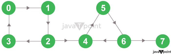

Figure 1: An Initial Directed Graph

The strongly connected components of the above graph will be: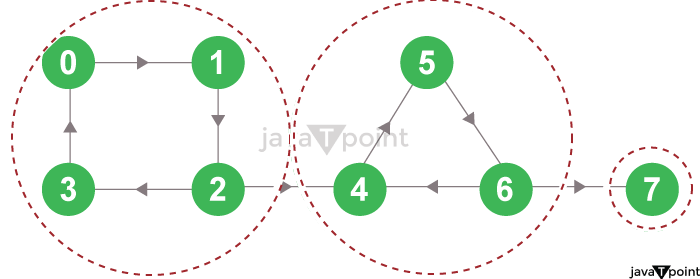

Figure 2: The Strongly Connected Components of the Directed Graph

As we can observe from the above figure, every node in the first strongly connected component reaches the other vertex through the directed path. And similar observations can be drawn for the second and third strongly connected components.

We can find these components using Kosaraju's Algorithm.

Understanding the Kosaraju's Algorithm

Kosaraju's Algorithm is centred on twice implementation of the depth-first search algorithm.

The complete procedure of this algorithm is divided into steps discussed below:

Step 1: Firstly, we will perform a depth first search on the complete graph.

We will start from node A, visit all its child nodes, and mark the selected node as visited. If the node leads to an already visited node, we will push the current node to the stack.

Figure 3.1: A Given Graph

For instance, in the given graph, we will start from node 0, visit node 1, node 2, and then node 3. Since node 3 leads to an already visited node, i.e., node 0, we will push the source node (i.e., node 3) into the stack.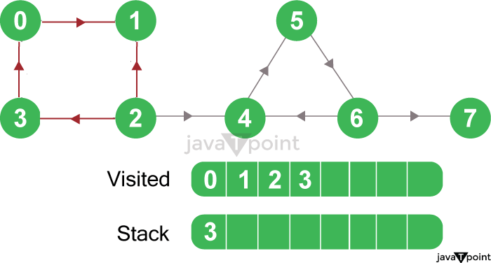

Figure 3.2: DFS on the Graph

We will then go to the previous node and visit its unvisited child nodes, i.e., node 4, node 5, node 6, and node 7, sequentially. Since we can't go anywhere from node 7, we will push it into the stack.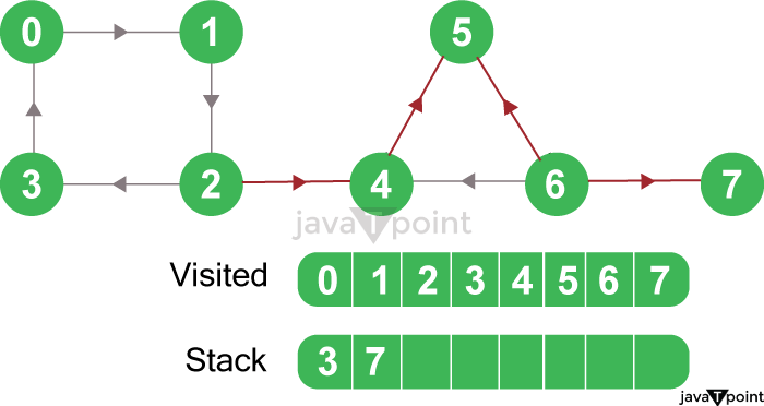

Figure 3.3: DFS on the Graph

We will now return to the previous node (i.e., node 6) and visit its child nodes. However, we will push it into the stack since all of its child nodes are already visited.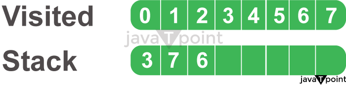

Figure 3.4: Stacking

In the similar way, a final stack is created.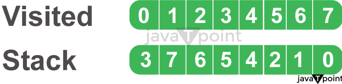

Figure 3.5: Final Stack

Step 2: Reversing the Original Graph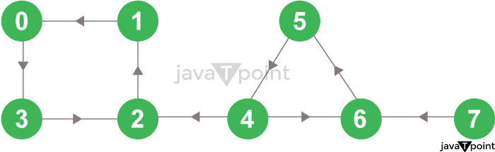

Figure 3.6: DFS on Reversed Graph

Step 3: Performing Depth-First Search on the Reversed Graph

We will now start from the top node of the stack and traverse through all its child nodes. Once the already visited node is reached, one strongly connected component is formed.

For instance, we will pop node 0 from the stack. Starting from node 0, we will traverse through its child nodes (node 0, node 1, node 2, node 3 in sequence) and mark them as visited so these visited nodes form one strongly connected component.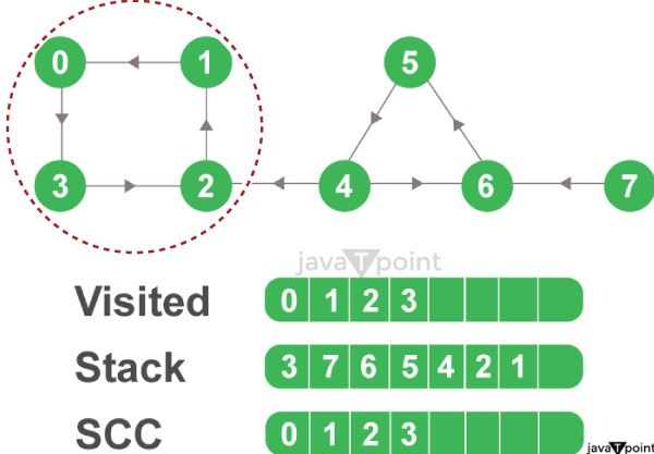

Figure 3.7: Start from Top and Traverse through All the Nodes

We will now go to stack and start popping the top node if it is already visited. Otherwise, we will select the top node from the stack and start traversing through its child nodes, as presented in the given figures.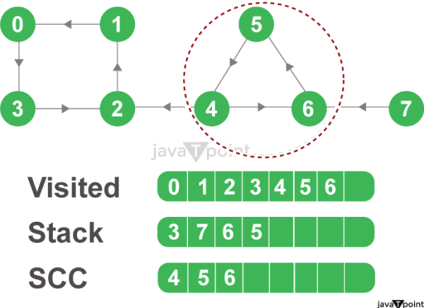

Figure 3.8: Pop the Top Node if Already Visited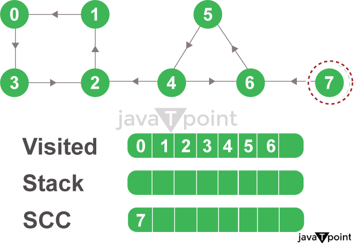

Figure 3.9: Strongly Connected Component

Step 4: Hence, the strongly connected components of the graph are as follows: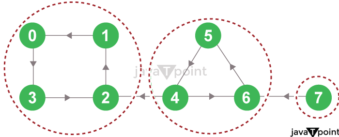

Figure 3.10: All Strongly Connected Components

Implementation of Kosaraju's Algorithm in Different Programming Languages

Now that we have successfully understood the concepts and working of Kosaraju's Algorithm, it is time to see its implementation in different programming languages like C++, and Python.

Code for Kosaraju's Algorithm in C++

The following is the implementation of Kosaraju's Algorithm in the C++ Programming Language:

File: example.cpp

// Kosaraju's Algorithm - Implementation in C++ to find strongly connected components

// including the required header files
#include <iostream>
#include <list>
#include <stack>

// using the standard namespace
using namespace std;

// defining the class
class DirectedGraph {
  // defining the required variables
  int N;  // number of variables
  list<int> *adj;   // empty list
  void fill_order(int a, bool visitedNodes[], stack<int> &Stack);  // method to push the elements in the stack
  void depth_first_search(int a, bool visitedNodes[]);   // method to perform depth first search   
   public:
    DirectedGraph(int N); // constructor for the graph creation
    void add_edge(int a, int d); // method to add edges into the graph
    void print_strongly_connected_components(); // method to print the strongly connected components
    DirectedGraph transpose(); // method to transpose nodes of the graph
};

// defining the constructor to create the graph
DirectedGraph :: DirectedGraph(int N) {
  this -> N = N;
  adj = new list<int>[N];
}

// defining the method to perform depth first search
void DirectedGraph :: depth_first_search(int a, bool visitedNodes[]) {
  visitedNodes[a] = true;
  cout << a << " ";

  list<int> :: iterator i;
  for (i = adj[a].begin(); i != adj[a].end(); ++i)
    if (!visitedNodes[*i])
      depth_first_search(*i, visitedNodes);
}

// defining the method to transpose nodes of the graph
DirectedGraph DirectedGraph :: transpose() {
  DirectedGraph graph(N);
  for (int a = 0; a < N; a++) {
    list<int>::iterator i;
    for (i = adj[a].begin(); i != adj[a].end(); ++i) {
      graph.adj[*i].push_back(a);
    }
  }
  return graph;
}

// defining the method to add edge into the graph
void DirectedGraph :: add_edge(int a, int d) {
  adj[a].push_back(d);
}

// defining the method to push elements into the stack
void DirectedGraph :: fill_order(int a, bool visitedNodes[], stack<int> &Stack) {
  visitedNodes[a] = true;

  list<int> :: iterator i;
  for (i = adj[a].begin(); i != adj[a].end(); ++i)
    if (!visitedNodes[*i])
      fill_order(*i, visitedNodes, Stack);

  Stack.push(a);
}

// defining the method print the strongly connected component
void DirectedGraph :: print_strongly_connected_components() {
  stack<int> Stack;

  bool *visitedNodes = new bool[N];
  for (int i = 0; i < N; i++)
    visitedNodes[i] = false;

  for (int i = 0; i < N; i++)
    if (visitedNodes[i] == false)
      fill_order(i, visitedNodes, Stack);

  DirectedGraph graph = transpose();

  for (int i = 0; i < N; i++)
    visitedNodes[i] = false;

  while (Stack.empty() == false) {
    int a = Stack.top();
    Stack.pop();

    if (visitedNodes[a] == false) {
      graph.depth_first_search(a, visitedNodes);
      cout << endl;
    }
  }
}

// main function
int main() {
  // instantiating the DirectedGraph() class to create a graph
  DirectedGraph graph(8);
  
  // adding edges to the graph
  graph.add_edge(0, 1);
  graph.add_edge(1, 2);
  graph.add_edge(2, 3);
  graph.add_edge(2, 4);
  graph.add_edge(3, 0);
  graph.add_edge(4, 5);
  graph.add_edge(5, 6);
  graph.add_edge(6, 4);
  graph.add_edge(6, 7);

  // printing a statement for the users
  cout << "The Strongly Connected Components of the Graph :\n";
  // calling the print_strongly_connected_components() method to print all the strongly connected components of the graph
  graph.print_strongly_connected_components();
}

Output:

The Strongly Connected Components of the Graph :
0 3 2 1
4 6 5
7

Explanation:

In the above snippet of code, we have included the required header files and used the standard namespace. We then defined a class as DirectedGraph. Inside this class, we have defined some variables and methods to serve different purposes in the program. We then defined a constructor to create a graph for the number of nodes. We have also defined the method to perform the depth-first search, where we will visit all the child nodes of the selected node and mark them visited. We then defined the method to transpose the nodes of the graph to reverse its order. We have also defined the method to add edges between the nodes to represent the directions in the graph. After that, we have defined the method to push the current node into the stack if it leads to visited nodes. We have also defined the method to print all the strongly connected components of the graph for the users. For the main function, we have instantiated the DirectedGraph() class and used its add_edge() method to add different edges to the graph. At last, we have printed a statement for the users and called the print_strongly_connected_components() method to print all the strongly connected components of the graph.

As a result, all the possible strongly connected components of the graph are printed for the users.

Code for Kosaraju's Algorithm in Python

The following is the implementation of Kosaraju's Algorithm in the Python Programming Language:

File: example.py

# Kosaraju's Algorithm - Implementation in Python to find strongly connected components

# importing the defaultdict class from the collections module
from collections import defaultdict

# defining the class
class DirectedGraph:
    # defining an initializing method
    def __init__(self, nodes):
        # defining variables
        self.N = nodes     # number of nodes
        self.directed_graph = defaultdict(list)    # empty list

    # defining the method to add edge into the graph
    def addEdge(self, a, d):
        self.directed_graph[a].append(d)

    # defining the method to perform depth first search
    def depthFirstSearch(self, d, visited_nodes):
        visited_nodes[d] = True
        print(d, end = ' ')
        for i in self.directed_graph[d]:
            if not visited_nodes[i]:
                self.depthFirstSearch(i, visited_nodes)

    # defining the method to push elements into the stack
    def fillOrder(self, d, visited_nodes, stack):
        visited_nodes[d] = True
        for i in self.directed_graph[d]:
            if not visited_nodes[i]:
                self.fillOrder(i, visited_nodes, stack)
        stack = stack.append(d)

    # defining the method to transpose nodes of the graph
    def transpose(self):
        graph = DirectedGraph(self.N)

        for i in self.directed_graph:
            for j in self.directed_graph[i]:
                graph.addEdge(j, i)
        return graph

    # defining the method print the strongly connected components
    def printStronglyConnectedComponents(self):
        stack = []
        visited_nodes = [False] * (self.N)

        for i in range(self.N):
            if not visited_nodes[i]:
                self.fillOrder(i, visited_nodes, stack)

        graph = self.transpose()

        visited_nodes = [False] * (self.N)

        while stack:
            i = stack.pop()
            if not visited_nodes[i]:
                graph.depthFirstSearch(i, visited_nodes)
                print(" ")

# main function
if __name__ == '__main__':
    # instantiating the DirectedGraph() class to create a graph
    graph = DirectedGraph(8)

    # adding edges to the graph
    graph.addEdge(0, 1)
    graph.addEdge(1, 2)
    graph.addEdge(2, 3)
    graph.addEdge(2, 4)
    graph.addEdge(3, 0)
    graph.addEdge(4, 5)
    graph.addEdge(5, 6)
    graph.addEdge(6, 4)
    graph.addEdge(6, 7)

    # printing a statement for the users
    print("The Strongly Connected Components of the Graph :")
    # calling the printStronglyConnectedComponents() method to print all the strongly connected components of the graph
    graph.printStronglyConnectedComponents()

Output:

The Strongly Connected Components of the Graph :
0 3 2 1
4 6 5
7

Explanation:

In the above snippet of code, we have imported defaultdict class from the collections library and defined a class as DirectedGraph. Inside this class, we have defined an initializing method to define and initialize some variables required in the program. We have then defined the method to add edges between the nodes to represent the directions in the graph. We have also defined the method to perform the depth-first search, where we will visit all the child nodes of the selected node and mark them visited. After that, we have defined the method to push the current node into the stack if it leads to visited nodes. We have also defined the method to transpose the nodes of the graph to reverse its order and the method to print all the strongly connected components of the graph for the users. For the main function, we have instantiated the DirectedGraph() class and used its addEdge() method to add different edges to the graph. At last, we have printed a statement for the users and called the printStronglyConnectedComponents() method to print all the strongly connected components of the graph.

As a result, all the possible strongly connected components of the graph are printed for the users.

Understanding the Time and Space Complexity of Kosaraju's Algorithm

Time Complexity: In Kosaraju Algorithm, there are mainly three steps that take place:

Calling the Depth-First Search: Time taken to perform Depth-First Search (DFS) on the graph exemplified by the adjacency list is O(V + E).
Reversing the Graph represented by the Adjacency list: To reverse the graph depicted with the help of the Adjacency list, we are required to iterate over the adjacency list, and the time taken for this process will be O(V).
Calling the Depth-First Search Again: The time taken to perform Depth-First Search (DFS) on the graph exemplified by the adjacency list is O(V + E).

Therefore, the total time taken to perform the above three steps in Kosaraju's Algorithm will be:

O(V + E) + O(V) + O(V + E) = O(V + E)

Hence, the time complexity of Kosaraju's Algorithm is O(V + E), where V is the number of nodes and E is the number of edges in the graph

Space Complexity: Since Kosaraju's Algorithm uses a stack to store the nodes while performing the first Depth-First Search (DFS), thus the space utilized by the stack will be equal to the size of the nodes of the graph.

Therefore, the space complexity of Kosaraju's Algorithm is O(N), where N is the number of nodes in the graph.

Advantages and Disadvantages of Kosaraju's Algorithm

The advantages of Kosaraju's Algorithm are that we can easily implement it using Depth-First Search (DFS), and it has a time complexity of O(V + E), where V is the number of nodes and E is the number of edges in the graph.
The disadvantages of this algorithm are that it requires storing the graph and its transposition in memory, which can be an issue for large graphs. Moreover, the algorithm is unsuitable for undirected graphs as it will identify all nodes belonging to a single Strongly Connected Component.

Applications of Strongly Connected Components

The following are some applications of Strongly Connected Components:

Strongly Connected Components (SCC) are generally utilized in Social Media Algorithms where SCC serves the purpose of knowing people with common interests and mutual friends.
Strongly Connected Components (SCC) are also utilized in Maps Algorithm in order to link the path with a similar origin and destination.
Strongly Connected Components (SCC) are also utilized in algorithms used for Vehicle Routing.

Alternatives of Kosaraju's Algorithm

In addition to Kosaraju's Algorithm, there are some other algorithms that are used to find strongly connected components in a directed graph. Some examples of such algorithms are Tarjan's Algorithm and the Path-Based Strong Component Algorithm.

Tarjan's Algorithm is similar to Kosaraju's Algorithm because it also utilizes Depth-First Search (DFS); however, it uses a different approach in order to identify Strongly Connected Components of the graph.
The Path-Based Strong Component Algorithm is a more recent algorithm that uses the approach of Dynamic Programming in identifying the Strongly Connected Components of the graph.

The Conclusion

In the above tutorial, firstly, we have understood the basic concepts of Strongly Connected Components of the Graph.
We then learned about Kosaraju's Algorithm with its working.
After that, we observed its implementation in programming languages like C++ and Python with proper outputs and explanations.
We have also understood the Time and Space Complexity of Dijkstra's Algorithm.
Finally, we have discussed the advantages and disadvantages of Dijkstra's algorithm and some real-life applications and understand its alternatives.

Next TopicFloyd-Warshall Algorithm

← prev next →