Travelling Salesman Problem

In the following tutorial, we will discuss the Travelling Salesman Problem with its solution and implementation in different programming languages using different approaches.

So, let's get started.

Understanding the Travelling Salesman Problem

The Travelling Salesman Problem (also known as the Travelling Salesperson Problem or TSP) is an NP-hard graph computational problem where the salesman must visit all cities (denoted using vertices in a graph) given in a set just once. The distances (denoted using edges in the graph) between all these cities are known. We are requested to find the shortest possible route in which the salesman visits all the cities and returns to the origin city.

Note:

There is a difference between Hamiltonian Cycle and TSP. The Hamiltonian Cycle problem is the problem where we have to find if there exists a tour that visits every city accurately once. However, in this problem, we already know that Hamiltonian Tour exists as the graph is complete, and in fact, there exist many such tours. Therefore, the problem is to find a minimum weight Hamiltonian Cycle.

Let us consider the following examples demonstrating the problem:

Example 1 of Travelling Salesman Problem

Input: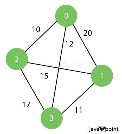

Output: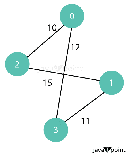

Example 2 of Travelling Salesman Problem

Input: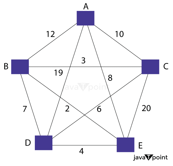

Output:

Minimum Weight Hamiltonian Cycle: EACBDE = 32

Solution of the Travelling Salesman Problem

In the following section, we will discuss different approaches that we will use to solve the problem and their implementations in different programming languages like C, C++, Java, and Python.

The following are some approaches that we are going to use:

Simple or Na�ve Approach
Dynamic Programming Approach
Greedy Approach

Let us now discuss the approaches mentioned above in detail:

Solving Travelling Salesman Problem using Simple Approach

In the following approach, we will solve the problem using the steps mentioned below:

Step 1: Firstly, we will consider City 1 as the starting and ending point. Since the route is cyclic, any point can be considered a starting point.

Step 2: As the second step, we will generate all the possible permutations of the cities, which are (n-1)!

Step 3: After that, we will find the cost of each permutation and keep a record of the minimum cost permutation.

Step 4: At last, we will return the permutation with minimum cost.

Implementation of Simple Approach to Solve Travelling Salesman Problem in Different Programming Languages

Now that we have successfully understood the steps for the simple approach to solve Travelling Salesman Problem, it is time to see its implementation in different programming languages like C++, Java, and Python.

Code Implementation in C++

The following is the implementation of the Travelling Salesman Problem's Algorithm in the C++ Programming Language:

File: TSP.cpp

// Travelling Salesman Problem - Simple Approach Implementation in C++ 

// including the required header file
#include <bits/stdc++.h>

// using the standard namespace
using namespace std;

// defining the constant number of nodes
#define V 4

// defining the function to return the minimum weight Hamiltonian cycle
int travelling_salesman_problem(int graph[][V], int n)
{
    // creating a vector to store the nodes
    vector<int> nodes;
    // iterating through defined number of nodes and pushing elements into the vector from the back if the current value is not equal to source node
    for (int i = 0; i < V; i++)
        if (i != n)
            nodes.push_back(i);

    // setting an initial value for minimum path as Integer's maximum value
    int minimumPath = INT_MAX;

    // do-while loop
    do {
        // setting an initial value of current path weight as 0
        int currentPathWeight = 0;
        int k = n;
        // iterating through the vector and incrementing the current path weight 
        for (int i = 0; i < nodes.size(); i++) {
            currentPathWeight += graph[k][nodes[i]];
            k = nodes[i];
        }
        currentPathWeight += graph[k][n];
 
        // updating the minimum path weight
        minimumPath = min(minimumPath, currentPathWeight);
    } while (
        next_permutation(nodes.begin(), nodes.end())
        );
    
    // returning the minimum path weight
    return minimumPath;
}

// main function
int main()
{   
    // defining the nodes of the graph
    int graph[][V] = {
        { 0, 12, 18, 24 },
        { 12, 0, 36, 28 },
        { 18, 36, 0, 32 },
        { 24, 28, 32, 0 }
        };

    // starting node
    int n = 0;

    // calling the travelling_salesman_problem() function
    int minimumPathWeight = travelling_salesman_problem(graph, n);

    // printing the result for the users
    cout << "Minimum Cost : " << minimumPathWeight << endl;
    return 0;
}

Output:

Minimum Cost : 90

Explanation:

In the above snippet of code, we have included the 'bits/stdc++.h' header file, used the standard namespace, and defined a constant value as V = 4 that represents the number of nodes in the graph. We have then defined the function to find the minimum weight Hamiltonian cycle cost as travelling_salesman_problem() that accepts a two-dimensional array representing the graph and an integer representing the starting node. Inside this function, we have created a vector in order to store the nodes from the graph. We have then iterated through the defined number of vertices using the for-loop and used the vector's push_back() method to push each element into the vector if it is not the source node. We have then set an initial value for minimum path weight as INT_MAX (maximum integer value). We then used the do-while loop to update the minimum path weight for all the possible permutations. Inside this loop, we have set an initial value of the current path weight as 0 and then iterated through the vector incrementing the current path weight according to the graph's edges. We have then updated the minimum path weight by comparing the current path weight and the stored value. We have then returned the resulting path weight and defined a main function. We have defined the graph inside the main function using the adjacency matrix and set a starting node. We have then called the travelling_salesman_problem() function to find the minimum weight Hamiltonian cycle cost and stored the returned value in a variable. At last, we have printed this variable for the users.

As a result, the minimum weight Hamiltonian cycle cost, i.e., 90, is printed for the users.

Code Implementation in Java

The following is the implementation of the Travelling Salesman Problem's Algorithm in the Java Programming Language:

File: TSP.java

// Travelling Salesman Problem - Simple Approach Implementation in Java

// importing the required library
import java.util.*;

// defining the class to solve Travelling Salesman Problem
class TSP{

    // initializing a constant value for number of nodes
    static int V = 4;

    // defining the method to find the minimum weight Hamiltonian Cycle
    static int travelling_salesman_problem(int graph[][], int n)
    {
        // creating an array to store the number of numbers
        ArrayList<Integer> nodes = new ArrayList<Integer>();

        // iterating through the number of nodes and adding elements into the array if the current value is not equal to source node
        for (int i = 0; i < V; i++)
            if (i != n)
                nodes.add(i);

        // setting an initial value for minimum path as Integer's maximum value 
        int minimumPath = Integer.MAX_VALUE;
        
        // do-while loop
        do
        {
            // setting an initial value of current path weight as 0
            int currentPathWeight = 0;
            int k = n;
            // iterating through the array and incrementing the current path weight
            for (int i = 0; i < nodes.size(); i++)
            {
                currentPathWeight += graph[k][nodes.get(i)];
                k = nodes.get(i);
            }
            currentPathWeight += graph[k][n];
            
            // updating the minimum path weight
            minimumPath = Math.min(minimumPath, currentPathWeight);

        } while (next_permutation(nodes));

        return minimumPath;
    }

    // defining the method to swap the elements of the array list
    public static ArrayList<Integer> swap(ArrayList<Integer> data, int leftElement, int rightElement){
        int temp = data.get(leftElement);
        data.set(leftElement, data.get(rightElement));
        data.set(rightElement, temp);
        return data;
    }

    // defining the method to reverse the data elements of the array list
    public static ArrayList<Integer> reverse(ArrayList<Integer> data, int leftElement, int rightElement)
    {
        while (leftElement < rightElement)
        {
            int temp = data.get(leftElement);
            data.set(leftElement++, data.get(rightElement));
            data.set(rightElement--, temp);
        }
        return data;
    }

    // defining the method to return the next permutation in the array list
    public static boolean next_permutation(ArrayList<Integer> data)
    {
        if (data.size() <= 1)
            return false;

        int last = data.size() - 2;
        while (last >= 0)   
        {
            if (data.get(last) < data.get(last + 1))
            {
                break;
            }
            last--;
        }
        if (last < 0)
            return false;

        int next_greater = data.size() - 1;
        for (int i = data.size() - 1; i > last; i--) {
            if (data.get(i) > data.get(last))
            {
                next_greater = i;
                break;
            }
        }
        data = swap(data, next_greater, last);
        data = reverse(data, last + 1, data.size() - 1);
        return true;
    }

    // main function
    public static void main(String args[])
    {
        // defining the nodes of the graph
        int graph[][] = {
            { 0, 12, 18, 24 },
            { 12, 0, 36, 28 },
            { 18, 36, 0, 32 },
            { 24, 28, 32, 0 }
            };

        // starting node
        int n = 0;

        // calling the travelling_salesman_problem() method
        int minimumPathWeight = travelling_salesman_problem(graph, n);
        
        // printing the result for the users
        System.out.print("Minimum Cost : ");
        System.out.print(minimumPathWeight);
        }
    }

Output:

Minimum Cost : 90

Explanation:

In the above snippet of code, we have imported everything from the 'java.util' library and defined the main class as TSP to solve the Travelling Salesman Problem. In this class, we have initialized a constant value as V = 4, which represents the total number of nodes in the graph. We have then defined the method to find the minimum weight Hamiltonian cycle cost as travelling_salesman_problem() that accepts a two-dimensional array representing the graph and an integer representing the starting node. Inside this function, we have created an integer array using ArrayList to store the nodes from the graph. We have then iterated through the defined number of vertices using the for-loop and used the add() method to add each element into the vector if it is not the source node. We have then set an initial value for the minimum path weight as Integer.MAX_VALUE (maximum integer value). We then used the do-while loop to update the minimum path weight for all the possible permutations. Inside this loop, we have set an initial value of the current path weight as 0 and then iterated through the array incrementing the current path weight according to the graph's edges. We have then updated the minimum path weight by comparing the current path weight and the stored value. We have then returned the resulting path weight. After that, we have defined a few more methods that will help us swap the elements of the array, reverse them, and to do permutations. We then defined the main function, creating the graph using the adjacency matrix and setting a starting node. Then, we called the travelling_salesman_problem() function to find the minimum weight Hamiltonian cycle cost and stored the returned value in a variable. At last, we have printed this variable for the users.

As a result, the minimum weight Hamiltonian cycle cost, i.e., 90, is printed for the users.

Code Implementation in Python

The following is the implementation of the Travelling Salesman Problem's Algorithm in the Python Programming Language:

File: TSP.py

# Travelling Salesman Problem - Simple Approach Implementation in Python

# importing the required modules
from itertools import permutations
from sys import maxsize

# defining a constant value for the number of nodes
V = 4

# defining the method to find the minimum weight Hamiltonian Cycle
def travelling_salesman_problem(graph, n):
    
    # creating an empty list to store the number of numbers
    nodes = []
    
    # iterating through the number of nodes and adding elements into the array if the current value is not equal to source node
    for i in range(V):
        if i != n:
            nodes.append(i)

    # setting an initial value for minimum path as Integer's maximum value
    minimumPath = maxsize
    
    # instantiating the permutations() class
    nextPermutation = permutations(nodes)
    
    # iterating through each permutation and updating the minimum path weight
    for i in nextPermutation:
        
        # initializing the current path weight as 0
        currentPathWeight = 0
        k = n
        
        # iterating through the list and incrementing the current path weight
        for j in i:
            currentPathWeight += graph[k][j]
            k = j
        currentPathWeight += graph[k][n]
        
        # updating the minimum path weight
        minimumPath = min(minimumPath, currentPathWeight)
        
    return minimumPath

# main function
if __name__ == "__main__":
    
    # defining the nodes of the graph
    graph = [
        [ 0, 12, 18, 24 ],
        [ 12, 0, 36, 28 ],
        [ 18, 36, 0, 32 ],
        [ 24, 28, 32, 0 ]
    ]
    
    # starting node
    n = 0
    
    # calling the travelling_salesman_problem() function
    minimumPathWeight = travelling_salesman_problem(graph, n)
    
    # printing the result for the users
    print("Minimum Cost :", minimumPathWeight)

Output:

Minimum Cost : 90

Explanation:

In the above snippet of code, we have imported the permutations class from the itertools module along with the maxsize variable from the sys module. We then initialized a constant value as V = 4, representing the total number of nodes in the graph. We have then defined the function to find the minimum weight Hamiltonian cycle cost as travelling_salesman_problem() that accepts a list representing the graph and an integer representing the starting node. Inside this function, we have created an empty list to store the nodes from the graph. We have then iterated through the defined number of vertices using the for-loop and used the append() method to add each element into the vector if it is not the source node. We have then set an initial value for the minimum path weight as maxsize (maximum integer value). We then instantiated the permutations() class for the number of nodes and used the for-loop to iterate through each permutation and update the minimum path weight accordingly. Inside this loop, we have set an initial value of the current path weight as 0 and then iterated through the list incrementing the current path weight according to the graph's edges. We have then updated the minimum path weight by comparing the current path weight and the stored value. We have then returned the resulting path weight. We then defined the main function, creating the graph and setting a starting node. Then, we called the travelling_salesman_problem() function to find the minimum weight Hamiltonian cycle cost and stored the returned value in a variable. At last, we have printed this variable for the users.

As a result, the minimum weight Hamiltonian cycle cost, i.e., 90, is printed for the users.

Time and Space Complexity of Travelling Salesman Problem Using Simple Approach

The Time Complexity of the Travelling Salesman Problem using the Simple or Na�ve Approach will be O(N!), where N is the number of cities.
The Space Complexity of the Travelling Salesman Problem using the Simple or Na�ve Approach will be O(1).

Solving Travelling Salesman Problem Using Dynamic Programming Approach

In the following approach, we will solve the problem using the steps mentioned below:

Step 1: In travelling salesman problem algorithm, we will accept a subset N of the cities that require to be visited, the distance among the cities, and starting city S as inputs. Each city is represented by a unique city id (let's say 1, 2, 3, 4, 5, ..., n).

Step 2: Let us consider 1 as the starting and ending point of the problem. For every other node V (except 1), we will calculate the minimum cost path having 1 as the starting point, V as the ending point, and all nodes appearing exactly once.

Step 3: Let the cost of this path cost (i), and the cost of the corresponding cycle would be cost(i) + distance(i, 1) where the distance(i, 1) from V to 1. Finally, we will return the minimum of all [cost(i) + distance(i, 1)] values.

The above procedure looks quite easy. However, the main question is how to calculate the cost(i)? In order to calculate the cost(i) with the help of Dynamic Programming, we are required to have some recursive relations in terms of sub-problems.

Let us define a term C(S, i) be the cost of the minimum cost path visiting each node in set S exactly once, beginning at 1 and ending at i. We will begin with all subsets of size 2 and calculate C(S, i) for all subsets S of size 3 and so on.

Note:

Node 1 must be present in every subset.

Implementation of Dynamic Programming Approach to Solve Travelling Salesman Problem in Different Programming Languages

We will now see the implementation of the Dynamic Programming solution using the Top-Down Recursive + Memorized approach in different programming languages like C++, Java, and Python.

To maintain the subsets, we can utilize the bitmasks in order to represent the remaining nodes in the subset. Since the operations are carried out faster using bits, and there are only a few nodes in the graph, bitmasks are better for usage.

For instance:

10100 signifies that nodes 2 and 4 are left in set for processing.
010010 signifies that nodes 1 and 4 are left in the subset.

Note:

Ignore the zeroth bit since the graph is 1-based.

Code Implementation in C++

The following is the implementation of the Travelling Salesman Problem's Algorithm in the C++ Programming Language:

File: TSP.cpp

// importing the 'iostream' header file
#include "iostream"

// using the standard namespace
using namespace std;

// defining the number of the nodes in the graph
const int V = 4;

// defining the maximum size to avoid overflow issue
const int MAX = 999999;

// graph[i][j] signifies the shortest distance to go from index i to index j
// we can calculate this matrix for any given graph using all-pair shortest path algorithms
int graph[V + 1][V + 1] = {
    { 0, 0, 0, 0, 0 },
    { 0, 0, 12, 18, 24 },
    { 0, 12, 0, 36, 28 },
    { 0, 18, 36, 0, 32 },
    { 0, 24, 28, 32, 0 }
    };

// memoization for top-down recursion
int memoize[V + 1][1 << (V + 1)];

// defining the recursive function to find the minimum weight Hamiltonian Cycle cost
int travelling_salesman_problem(int i, int mask)
{	
    // defining the base case
    // if only ith bit and first bit is set in the mask,
    // it means we have visited all other nodes already
    if (mask == ((1 << i) | 3))
        return graph[1][i];
    // performing memoization
    if (memoize[i][mask] != 0)
        return memoize[i][mask];

    // initializing the minimum cost as the Maximum integer value
    int minimumCost = MAX;

    // we have to travel all nodes j in mask and end the path at ith node so for every node j
    // in mask, recursively estimate the cost of travelling all nodes in mask except i and
    // then travel back from node j to node i taking the shortest path take the minimum of
    // all possible j nodes
    for (int j = 1; j <= V; j++)
        if ((mask & (1 << j)) && j != i && j != 1)
            minimumCost = std::min(minimumCost, travelling_salesman_problem(j, mask & (~(1 << i))) + graph[j][i]);
    return memoize[i][mask] = minimumCost;
}

// main function
int main()
{
    // defining and initializing the resultant cost as maximum Integer value
    int cost = MAX;

    // using the for-loop to iterate through the nodes
    for (int i = 1; i <= V; i++)
        // try to go from node 1 visiting all nodes in
        // between to i then return from i taking the
        // shortest route to 1
        cost = std::min(cost, travelling_salesman_problem(i, (1 << (V + 1)) - 1) + graph[i][1]);

    // printing the total cost for the users
    cout << "Minimum Cost : " << cost;

    return 0;
}

Output:

Minimum Cost : 90

Explanation:

In the above code snippet, we included the iostream header file and used the standard namespace. We then defined a constant value to represent the total number of vertices, the maximum integer size to avoid overflow issues, a graph, and a matrix to perform memoization for the top-down recursion approach. We have then defined the function as travelling_salesman_problem() that accepts two parameters - the first parameter is iterable, and the second one is the bitmask. Inside this function, we have defined a base case for the recursion, which will execute only when the current and first bit is set in the mask, implying that all other nodes have already been visited. After that, we performed memorization and initialized the minimum cost as the maximum integer value. We then used the for-loop to iterate through all the nodes in the mask. We recursively calculated the cost of travelling the nodes in the mask except the selected one and then travelling back to starting node by taking the shortest possible path. For the main function, we have initialized the resultant cost as the maximum integer value and used the for-loop to iterate through the nodes of the graph and calculate the new minimum cost by calling the travelling_salesman_problem() function for that particular node and set the minimum cost value as the resultant cost. At last, we have printed the result for the users.

As a result, the minimum weight Hamiltonian cycle cost, i.e., 90, is printed for the users.

Code Implementation in Java

The following is the implementation of the Travelling Salesman Problem's Algorithm in the Java Programming Language:

File: TSP.java

// Travelling Salesman Problem - Dynamic Programming Approach Implementation in Java

// defining the class to solve Travelling Salesman Problem
public class TSP {
    // defining the number of the nodes in the graph
    static int V = 4;

    // defining the maximum size to avoid overflow issue
    static int MAX_INT = 999999;

    // graph[i][j] signifies the shortest distance to go from index i to index j
    // we can calculate this matrix for any given graph using all-pair shortest path algorithms
    static int[][] graph = {
        { 0, 0, 0, 0, 0 },
        { 0, 0, 12, 18, 24 },
        { 0, 12, 0, 36, 28 },
        { 0, 18, 36, 0, 32 },
        { 0, 24, 28, 32, 0 }
    };

    // memoization for top-down recursion
    static int[][] memoize = new int[V + 1][1 << (V + 1)];

    // defining the recursive function to find the minimum weight Hamiltonian Cycle cost
    static int travelling_salesman_problem(int i, int mask)
    {
        // defining the base case
        // if only ith bit and first bit is set in the mask,
        // it means we have visited all other nodes already
        if (mask == ((1 << i) | 3))
            return graph[1][i];
        // performing memoization
        if (memoize[i][mask] != 0)
            return memoize[i][mask];

        // initializing the minimum cost as the Maximum integer value
        int minimumCost = MAX_INT;

        // we have to travel all nodes j in mask and end the path at ith node so for every node j
        // in mask, recursively estimate the cost of travelling all nodes in mask except i and
        // then travel back from node j to node i taking the shortest path take the minimum of
        // all possible j nodes
        for (int j = 1; j <= V; j++)
            if ((mask & (1 << j)) != 0 && j != i && j != 1)
                minimumCost = Math.min(minimumCost, travelling_salesman_problem(j, mask & (~(1 << i))) + graph[j][i]);
        return memoize[i][mask] = minimumCost;
    }

    // main function
    public static void main(String[] args)
    {
        // defining and initializing the resultant cost as maximum Integer value
        int cost = MAX_INT;

        // using the for-loop to iterate through the nodes
        for (int i = 1; i <= V; i++)
            // try to go from node 1 visiting all nodes in
            // between to i then return from i taking the
            // shortest route to 1
            cost = Math.min(cost, travelling_salesman_problem(i, (1 << (V + 1)) - 1) + graph[i][1]);

        // printing the total cost for the users
        System.out.println( "Minimum Cost : " + cost );
    }
}

Output:

Minimum Cost : 90

Explanation:

In the above code snippet, we defined a class as TSP. Within this class, we defined a constant value to represent the total number of vertices, the maximum integer size to avoid overflow issues, a graph, and a matrix to perform memoization for the top-down recursion approach. We have then defined the function as travelling_salesman_problem() that accepts two parameters - the first parameter is iterable, and the second one is the bitmask. Inside this function, we have defined a base case for the recursion, which will execute only when the current and first bit is set in the mask, implying that all other nodes have already been visited. After that, we performed memorization and initialized the minimum cost as the maximum integer value. We then used the for-loop to iterate through all the nodes in the mask. We recursively calculated the cost of travelling the nodes in the mask except the selected one and then travelling back to starting node by taking the shortest possible path. For the main function, we have initialized the resultant cost as the maximum integer value and used the for-loop to iterate through the nodes of the graph and calculate the new minimum cost by calling the travelling_salesman_problem() function for that particular node and set the minimum cost value as the resultant cost. At last, we have printed the result for the users.

As a result, the minimum weight Hamiltonian cycle cost, i.e., 90, is printed for the users.

Code Implementation in Python

The following is the implementation of the Travelling Salesman Problem's Algorithm in the Python Programming Language:

File: TSP.py

# Travelling Salesman Problem - Dynamic Programming Approach Implementation in Python

# defining the number of the nodes in the graph
V = 4

# graph[i][j] signifies the shortest distance to go from index i to index j
# we can calculate this matrix for any given graph using all-pair shortest path algorithms
graph = [
    [0, 0, 0, 0, 0],
    [0, 0, 12, 18, 24],
    [0, 12, 0, 36, 28],
    [0, 18, 36, 0, 32],
    [0, 24, 28, 32, 0]
    ]

# memoization for top-down recursion
memoize = [[-1] * (1 << (V + 1)) for _ in range(V + 1)]

# defining the recursive function to find the minimum weight Hamiltonian Cycle cost
def travelling_salesman_problem(i, mask):
    # defining the base case
    # if only ith bit and first bit is set in the mask,
    # it means we have visited all other nodes already
    if mask == ((1 << i) | 3):
        return graph[1][i]

    # performing memoization
    if memoize[i][mask] != -1:
        return memoize[i][mask]

    # initializing the minimum cost as the Maximum integer value
    minimumCost = 10 ** 9

    # we have to travel all nodes j in mask and end the path at ith node so for every node j
    # in mask, recursively estimate the cost of travelling all nodes in mask except i and
    # then travel back from node j to node i taking the shortest path take the minimum of
    # all possible j nodes
    for j in range(1, V + 1):       
        if (mask & (1 << j)) != 0 and j != i and j != 1:
            minimumCost = min(minimumCost, travelling_salesman_problem(j, mask & (~(1 << i))) + graph[j][i])
    memoize[i][mask] = minimumCost # storing the minimum value
    return minimumCost

# main function
if __name__ == "__main__":
    #  defining and initializing the resultant cost as maximum Integer value
    cost = 10 ** 9
    
    # using the for-loop to iterate through the nodes
    for i in range(1, V + 1):
        # try to go from node 1 visiting all nodes in
        # between to i then return from i taking the
        # shortest route to 1
        cost = min(cost, travelling_salesman_problem(i, (1 << (V + 1)) -1) + graph[i][1])

    # printing the total cost for the users
    print( "Minimum Cost : " + str(cost) )

Output:

Minimum Cost : 90

Explanation:

In the above code snippet, we defined a constant value to represent the total number of vertices, a graph, and a matrix to perform memoization for the top-down recursion approach. We have then defined the function as travelling_salesman_problem() that accepts two parameters - the first parameter is iterable, and the second one is the bitmask. Inside this function, we have defined a base case for the recursion, which will execute only when the current and first bit is set in the mask, implying that all other nodes have already been visited. After that, we performed memorization and initialized the minimum cost as the maximum integer value. We then used the for-loop to iterate through all the nodes in the mask. We recursively calculated the cost of travelling the nodes in the mask except the selected one and then travelling back to starting node by taking the shortest possible path. For the main function, we have initialized the resultant cost as the maximum integer value and used the for-loop to iterate through the nodes of the graph and calculate the new minimum cost by calling the travelling_salesman_problem() function for that particular node and set the minimum cost value as the resultant cost. At last, we have printed the result for the users.

As a result, the minimum weight Hamiltonian cycle cost, i.e., 90, is printed for the users.

Time and Space Complexity of Travelling Salesman Problem Using Dynamic Programming Approach

The Time Complexity of the Travelling Salesman Problem using the Dynamic Programming Approach will be O(N²* 2^N), where O(N * 2^N) are maximum number of unique sub-problems in recursion and O(N) for transition (through for-loop) in every nodes.
The Space Complexity of the Travelling Salesman Problem using the Dynamic Programming Approach will be O(N * 2^N), where N is the number of nodes.

Solving Travelling Salesman Problem Using Greedy Approach

In the following approach, we will solve the problem using the steps mentioned below:

Step 1: First of all, we will create two primary data holders - The first data holder will be the list to store the indices of the cities in terms of the input matrix of distances between the cities, and the second one will be the array to store the result.

Step 2: For the second step, we will traverse through the given adjacency matrix for all the cities and update the cost by checking if the cost of reaching any city from the current city is lower than the current cost.

Step 3: At last, we will generate the minimum path cycle with the help of the above step and return their minimum cost.

Implementation of Greedy Approach to Solve Travelling Salesman Problem in Different Programming Languages

Now that we have successfully understood the above procedure to solve the Travelling Salesman Problem using Greedy Approach, it is time to see its implementation in different programming languages like C++, Java, and Python.

Code Implementation in C++

The following is the implementation of the Travelling Salesman Problem's Algorithm in the C++ Programming Language:

File: TSP.cpp

// Travelling Salesman Problem - Greedy Approach Implementation in C++

// including the required library
#include "bits/stdc++.h"

// using the standard namespace
using namespace std;

// defining the function to find the minimum weight Hamiltonian Cycle cost
void travelling_salesman_problem(vector<vector<int>> graph)
{
    // initializing some variables
    int cost = 0;
    int count = 0;
    int j = 0, i = 0;
    int minimumCost = INT_MAX;
    map<int, int> visitedRoutes;
    visitedRoutes[0] = 1;
    int route[graph.size()];

    // using the while loop to iterate through the elements of the given graph
    while (i < graph.size() && j < graph[i].size())
    {   
        // breaking if the count value exceeds the size of the graph
        if (count >= graph[i].size() - 1)
        {
            break;
        }
        // if the index j is not equals to index i and the selected element at index j is 0
        if (j != i && (visitedRoutes[j] == 0))
        {
            // if the value is lower than the current minimum cost
            if (graph[i][j] < minimumCost)
            {
                // updating the minimum cost and incrementing the route count
                minimumCost = graph[i][j];
                route[count] = j + 1;
            }
        }
	  // incrementing the index j value by 1
        j++;
        
        // if the index j is equal to the size of the graph
        if (j == graph[i].size())
        {
            // updating the cost by adding the minimum cost to the current cost 
            cost += minimumCost;
            // setting the minimum cost as maximum integer value
            minimumCost = INT_MAX;
            // updating the route as 1 in the visitedRoutes[] array
            visitedRoutes[route[count] - 1] = 1;
            // initializing the index j equals to 0
            j = 0;
            // initializing the index i as the route[count] - 1
            i = route[count] - 1;
            // incrementing the count value by 1
            count++;
        }
    }
    // setting the index i as route[count -1] - 1
    i = route[count - 1] - 1;

    // using the for-loop to iterate through the graph
    for (j = 0; j < graph.size(); j++)
    {
        // if the index i is not equals to j and the value of the current element of the graph is less than the minimum cost
        if ((i != j) && graph[i][j] < minimumCost)
        {
            // updating the minimum cost and selected route value
            minimumCost = graph[i][j];
            route[count] = j + 1;
        }
    }

    // adding the final evaluated minimum cost to the total cost
    cost += minimumCost;

    // printing the total cost for the users
    cout << "Minimum Cost : " << (cost);
}

// main function
int main()
{
    // defining the graph
    vector<vector<int>> graph = {
        { -1, 12, 18, 24 },
        { 12, -1, 36, 28 },
        { 18, 36, -1, 32 },
        { 24, 28, 32, -1 }
        };

    // calling the travelling_salesman_problem() function to find the minimum weight Hamiltonian Cycle cost
    travelling_salesman_problem(graph);
    return 0;
}

Output:

Minimum Cost : 90

Explanation:

In the above snippet of code, we included the 'bits/stdc++.h' header file and used the standard namespace. We have then defined the function as travelling_salesman_problem(), which accepts a two-dimensional array as its parameter. Inside this function, we have defined some variables initializing them with some initial values. We then used the while loop to iterate through the graph and calculate the minimum cost. We have also included a break statement if the count exceeds the size of the graph. We updated the minimum cost value along with the route if the selected value from the graph is lower than the current minimum cost. We have also updated the total cost by adding the final minimum cost and setting the variables to their initial values. We then used the for-loop to generate the minimum path cycle by evaluating the total minimum cost and printed the result for the users. In the main function, we have defined the graph using the two-dimensional vector and called the travelling_salesman_problem() function to find the minimum weight Hamiltonian cycle cost.

As a result, the minimum weight Hamiltonian cycle cost, i.e., 90, is printed for the users.

Code Implementation in Java

The following is the implementation of the Travelling Salesman Problem's Algorithm in the Java Programming Language:

File: TSP.java

// Travelling Salesman Problem - Greedy Approach Implementation in Java

// importing the required library
import java.util.*;

// defining the class to solve Travelling Salesman Problem
public class TSP {

    // defining the method to find the minimum weight Hamiltonian Cycle
    static void travelling_salesman_problem(int[][] graph)
    {
        // initializing some variables
        int cost = 0;
        int count = 0;
        int j = 0, i = 0;
        int minimumCost = Integer.MAX_VALUE;
        List<Integer> visitedRoutes = new ArrayList<>();
        visitedRoutes.add(0);
        int[] route = new int[graph.length];

        // using the while loop to iterate through the elements of the given graph
        while (i < graph.length && j < graph[i].length)
        {
            // breaking if the count value exceeds the size of the graph
            if (count >= graph[i].length - 1)
            {
                break;
            }
            // if the index j is not equals to index i and the selected element at index j is 0
            if (j != i && !(visitedRoutes.contains(j)))
            {
                // if the value is lower than the current minimum cost
                if (graph[i][j] < minimumCost) {
                    // updating the minimum cost and incrementing the route count
                    minimumCost = graph[i][j];
                    route[count] = j + 1;
                }
            }
            // incrementing the index j value by 1
            j++;
            
            // if the index j is equal to the size of the graph
            if (j == graph[i].length)
            {
                // updating the cost by adding the minimum cost to the current cost
                cost += minimumCost;
                // setting the minimum cost as maximum integer value
                minimumCost = Integer.MAX_VALUE;
                // updating the route as 1 in the visitedRoutes[] array
                visitedRoutes.add(route[count] - 1);
                // initializing the index j equals to 0
                j = 0;
                // initializing the index i as the route[count] - 1
                i = route[count] - 1;
                // incrementing the count value by 1
                count++;
            }
        }
        // setting the index i as route[count -1] - 1
        i = route[count - 1] - 1;
        
        // using the for-loop to iterate through the graph
        for (j = 0; j < graph.length; j++)
        {
            // if the index i is not equals to j and the value of the current element of the graph is less than the minimum cost
            if ((i != j) && graph[i][j] < minimumCost)
            {
                // updating the minimum cost and selected route value
                minimumCost = graph[i][j];
                route[count] = j + 1;
            }
        }

        // adding the final evaluated minimum cost to the total cost
        cost += minimumCost;

        // printing the result for the users
        System.out.print("Minimum Cost : ");
        System.out.println(cost);
    }

    // main function
    public static void main(String[] args)
    {
        // defining the graph
        int[][] graph = {
            { -1, 12, 18, 24 },
            { 12, -1, 36, 28 },
            { 18, 36, -1, 32 },
            { 24, 28, 32, -1 }
        };

        // calling the travelling_salesman_problem() function to find the minimum weight Hamiltonian Cycle cost
        travelling_salesman_problem(graph);
    }
}

Output:

Minimum Cost : 90

Explanation:

In the above snippet of code, we have imported everything from the 'java.util' library and defined the main class as TSP to solve the Travelling Salesman Problem. In this class, we have defined the function as travelling_salesman_problem(), which accepts a two-dimensional array as its parameter. Inside this function, we have defined some variables initializing them with some initial values. We then used the while loop to iterate through the graph and calculate the minimum cost. We have also included a break statement if the count exceeds the size of the graph. We updated the minimum cost value along with the route if the selected value from the graph is lower than the current minimum cost. We have also updated the total cost by adding the final minimum cost and setting the variables to their initial values. We then used the for-loop to generate the minimum path cycle by evaluating the total minimum cost and printed the result for the users. In the main function, we have defined the graph and called the travelling_salesman_problem() function to find the minimum weight Hamiltonian cycle cost.

As a result, the minimum weight Hamiltonian cycle cost, i.e., 90, is printed for the users.

Code Implementation in Python

The following is the implementation of the Travelling Salesman Problem's Algorithm in the Python Programming Language:

File: TSP.py

# Travelling Salesman Problem - Greedy Approach Implementation in Python

# defining the function to find the minimum weight Hamiltonian Cycle cost
def travelling_salesman_problem(graph):

    # defining and initializing some variables
    cost = 0
    count = 0
    i = 0
    j = 0
    minimumCost = 999999999
    visitedRoutes = {}
    visitedRoutes[0] = 1
    route = [0] * len(graph)

    # using the while loop to iterate through the elements of the graph
    while i < len(graph) and j < len(graph[i]):
        
        # breaking if the count value exceeds the size of the graph
        if count >= len(graph[i]) - 1:
            break
        
        # if the index j is not equals to index i and the selected element at index j is not in visitedRoutes[] list
        if j != i and j not in visitedRoutes:
            # if the value is lower than the current minimum cost
            if graph[i][j] < minimumCost:
                # updating the minimum cost and incrementing the route count
                minimumCost = graph[i][j]
                route[count] = j + 1
        # incrementing the index j value by 1
        j += 1
        
        # if the index j is equal to the size of the graph
        if j == len(graph[i]):
            # updating the cost by adding the minimum cost to the current cost
            cost += minimumCost 
            # setting the minimum cost as a higher integer value
            minimumCost = 999999999 
            # updating the route as 1 in the visitedRoutes[] list
            visitedRoutes[route[count] - 1] = 1 
            # initializing the index j equals to 0
            j = 0
            # initializing the index i as the route[count] - 1
            i = route[count] - 1 
            # incrementing the count value by 1
            count += 1
    
    # setting the index i as route[count -1] - 1
    i = route[count - 1] - 1 

    # using the for-loop to iterate through the graph
    for  j in range(0, len(graph)):
        # if the index i is not equals to j and the value of the current element of the graph is less than the minimum cost
        if i != j and graph[i][j] < minimumCost:
            # updating the minimum cost and selected route value
            minimumCost = graph[i][j]
            route[count] = j + 1 
    
    # adding the final evaluated minimum cost to the total cost
    cost += minimumCost 
    print("Minimum Cost :", cost)

# main function 
if __name__ == '__main__':
    
    # defining the graph
    graph =  [
        [-1, 12, 18, 24],
        [12, -1, 36, 28],
        [18, 36, -1, 32],
        [24, 28, 32, -1]
        ]
    
    # calling the travelling_salesman_problem() function to find the minimum weight Hamiltonian Cycle cost
    travelling_salesman_problem(graph)

Output:

Minimum Cost : 90

Explanation:

In the above snippet of code, we have defined the main class as TSP to solve the Travelling Salesman Problem. In this class, we have defined the function as travelling_salesman_problem(), which accepts a two-dimensional list as its parameter. Inside this function, we have defined some variables initializing them with some initial values. We then used the while loop to iterate through the graph and calculate the minimum cost. We have also included a break statement if the count exceeds the size of the graph. We updated the minimum cost value along with the route if the selected value from the graph is lower than the current minimum cost. We have also updated the total cost by adding the final minimum cost and setting the variables to their initial values. We then used the for-loop to generate the minimum path cycle by evaluating the total minimum cost and printed the result for the users. In the main function, we have defined the graph and called the travelling_salesman_problem() function to find the minimum weight Hamiltonian cycle cost.

As a result, the minimum weight Hamiltonian cycle cost, i.e., 90, is printed for the users.

Time and Space Complexity of Travelling Salesman Problem Using Greedy Approach

The Time Complexity of the Travelling Salesman Problem using the Greedy Approach will be O(N² * log N), where N is the number of cities.
The Space Complexity of the Travelling Salesman Problem using the Greedy Approach will be O(N).

Next TopicKosaraju's Algorithm

← prev next →