PowerPivot in Microsoft Excel

It was well known that the respective "PowerPivot" is primarily considered as a popular Add-In that is available just under Microsoft Excel and this could be efficiently used to import various data sets with millions or trillions of rows from various other sources as well. Despite of this, it also helps in performing the quick data analysis while handling large data sets present under the Microsoft Excel in an effective manner.

Add-in feature was first introduced in the Microsoft Excel version 2010 and then after that it can be made as a native feature under 2013 onwards versions of Microsoft Excel. The power that PowerPivot possesses lies in its own data models, which can be considered the "databases."

Moreover, the data models are nothing but the respective data tables that are very much similar to those which we effectively use in SQL (Structured Query Language), and we can also slice and dice with these data tables, respectively. Inspite of this we can create relationships between them, and then we are required to combine those different data tables to create calculated columns for analysis in an advanced format, obviously for advanced reporting as well. And we can consider this as a "pocket database" which are available under Microsoft Excel and ideally in the hands of users respectively.

What is the difference between PowerPivot and Pivot Table in Microsoft Excel?

In Microsoft Excel both Power Pivot and Pivot Table are valuable tools for performing data analysis in Microsoft Excel, respectively. The pivot table holds good for quick and simple data summarization of the particular data set from a single source. On the other hand, the respective power pivot enables an individual to handle larger data sets, allowing an individual to take data from multiple sources effectively.

Deciding which one to pick usually depends upon the level of analysis which we need and how much familiar we are with the data modeling and the DAX expressions.

What is Traditional Pivot Table in Microsoft Excel?

It is well known that a traditional pivot table is a powerful data summarization tool available in the Microsoft Excel which can be used for the purpose of analyzing the datasets and find out the insights from it quickly. It also allows us to represent data by rows, columns, values, and filters to simplify the various complex data sets, making it easy for comparison and analysis. They are responsible for generating meaningful reports without using complex formulas or coding.

How can one easily Access the Traditional Pivot Table in Microsoft Excel?

If we want to access the traditional Pivot Table in Microsoft Excel, then in that scenario we are required to follow the steps below effectively.

Step 1: Firstly we must need to select the data, and then go to the "Insert" Tab and click on the "Pivot Table," which is present under the "Tables" group.

Step 2: Now in this step, we must need to select "From Table/Range" and then will specify the data range and the destination cell as well. By doing so, the pivot table will get appear on our screen effectively.

Step 3: At last we are required to make use of the "PivotTable Fields" pane for the purpose of organizing the fields by rows, columns, values, as well as by filters.

When to make use of the Traditional Pivot Table in Microsoft Excel?

We can make use of the Traditional Pivot Table in Microsoft Excel for the following reasons as well:

1. We can make use of the Traditional Pivot Table for the purpose of converting a large as well as the complex data sets into concise and understandable summaries.
2. With the help of the Traditional Pivot Table we can generate graphs, charts and report to effectively visualize the data.
3. In case we want to create data groups by categorizing and performing calculations such as sums, averages, counts, and percentages, respectively.
4. It can also be used to perform data analysis and make decisions based upon identified patterns, outliers, and anomalies in the selected data.

What is meant by Power Pivot in Microsoft Excel

It was well known that the respective Power Pivot is an advanced feature which is available in Microsoft Excel and can be used to perform data analysis. It lets a user's handle a large data set, perform complex calculations, and create interactive reports within Microsoft Excel. Unlike regular Excel sheets, PowerPivot make use of in-memory computing to manage out the millions of data rows.

How one can easily access the Power Pivot in Microsoft Excel?

If we are required to access the Power Pivot in Microsoft Excel, we need to enable the Power Pivot in Excel sheet by following the steps mentioned below.

Step 1: We must need to go to the "File" > "Options" > "Add-Ins."

Step 2: After that, we need to select "COM Add-ins" in the "Manage" options and click on the "GO" option respectively.

Step 3: Now, in this step, we are required to select the "Microsoft Office Power Pivot for Excel" and after that we will be clicking on the "OK" option.

Step 4: And on the Power Pivot tab, we will be selecting the "Add to Data Model" and then will import data from various sources such as Excel, databases, etc.

Purpose of Using PowerPivot in Microsoft Excel

The main purpose of using the "PowerPivot" is just about providing a method to summarize a large amount of data effectively, as it makes the data quite simple and easy to understand due to which a user can easily analyze huge amount of the numerical data in detail.

So let us now understand this by using some different examples where the PowerPivot can be treated as a useful tool:

• PowerPivot is useful while creating a List of Employees for various Departments: We all know that the respective "pivot" is known for automatically performing the calculations. So to understand it in a better way let us assume a scenario in which the user has a list of employees who belong to several different departments, and the respective user wants to sort the data by the name of each department and the counts of employees; if perform manually by any individual then it will take time and create headache. But, by creating the pivot table, the data can be sorted by the name of each department and the names of the employees under the department name.
• It is very useful while comparing the Sales Data. We will be taking scenario in which a user required to maintain a large sales data based on the month, and it basically contains several different products, and the respective user needs to analyze which product has been bringing the most busk. Though it can be done manually, but it will take a lot of time to do it. Instead, we can do it using the pivot table in just a few seconds.

Features of Excel Power Pivot

The various features of Power Pivot in Microsoft Excel are as follows:

1. It makes use of the Data Analysis Expressions (DAX): The powered pivot uses the data analysis expression or DAX as the expression language, which will helps

us to extend the data manipulation capabilities of Excel to allow more sophisticated as well as complex grouping, calculation, and performing out the analysis effectively that in turns helps to maintain the large sets of the data.

2. Multi-Core Processor: The other most important feature of power pivot is none other than the feature of multi-core processing as well as the memory gigabytes, which can be efficiently used to perform faster calculations as well as for processing out thousands of rows in just some seconds respectively, and also with the help of the "compression algorithms," it is much possible to load a large data into the memory.

3. Data can be easily imported from Multiple Sources: The respective power pivot allows the particular user to import as well as combine the data from multiple sources, and the data can be easily sourced from any location for extensive data analysis on the desktop respectively.

4. Security and Management Feature: The other most important feature of PowerPivot primarily includes security and management features, which allow an IT manager to measure and control the shared applications to assure security.

5. It is considered a Helpful Tool Editing Process: With the help of a power pivot, the user can easily edit the table manually while just looking at the sample of the data. There can be up to five rows of data in the selected table, and with this feature, a user can efficiently create and edit out the data at a faster speed and with accuracy.

Head to Head comparison between the PowerPivot and Pivot Table in Microsoft Excel

Let us now see the Head-to-head difference between the PowerPivot and Pivot Table in Microsoft Excel.

How to Activate PowerPivot Add-ins Under Microsoft Excel?

Power Pivot is an important feature in Microsoft Excel which enables us to import millions of rows of data from the multiple data sources into a single Excel workbook. So, let us now look at the below-mentioned step to achieve the concept of PowerPivot in our Excel sheet.

Step 1: We are required to open an Excel file, where we need to click on the File tab at the upper Excel worksheet ribbon. And then Go to Options.

Step 2: Once we click on the Options button, we will be encountered with the window, "Excel Options," with a list of different Microsoft Excel options, and we are about click on the Add-ins option from that list to access all the add-ins in the Excel sheet.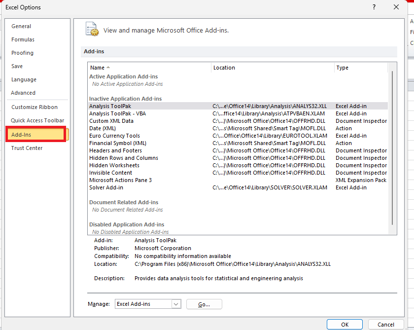

Step 3: Now we can find the Manage: section dropdown on the below side of this window, so in that dropdown menu, we are required to select the COM Add-ins and will then click on the GO button as well.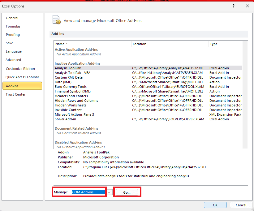

Step 4: After performing the above step, we will encounter the COM Add-ins dialog box on our screen, in which we are required to select Microsoft PowerPivot for Excel and proceed further by just clicking the OK button.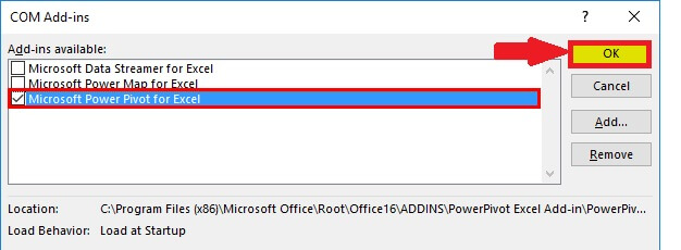

Once we enable this add-in, we can see a new option that will be added up in the respective Excel ribbon known as "PowerPivot," as depicted in the image mentioned- below: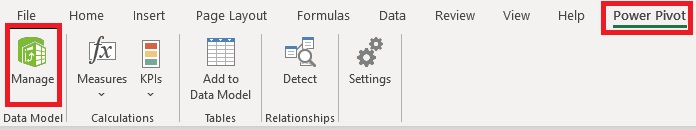

To launch the respective PowerPivot, we must also click on the "Manage option" that is present under the Data Model section in the PowerPivot tab. The PowerPivot window will look like the one in the image mentioned below: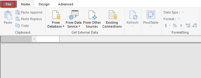

How can one easily import Datasets under PowerPivot Microsoft Excel?

In this, we can easily import data from the various multiple resources under the power pivot, which makes it awesome to work on, and it will also allow us to import data from SQL, ORACLE DB, etc. At the same time, we can import data through .xls/xlsx and .txt files. We will import a text data file under PowerPivot effectively.

To achieve this effectively, we will be following the below-mentioned steps very carefully:

Step 1: First of all, under PowerPivot for the Excel sheet, we are required to click on the From Other Sources button in the Get External Data section and doing this will open up a series of external sources from where we can easily fetch the data that are present just under the PowerPivot section as well.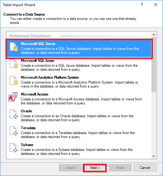

Step 2: Now we will be navigating to the end by using the scroll bar, and there, we can see an option through which we can import data from a text file. After that we will be clicking on that option and hit the Next button to proceed with the next step.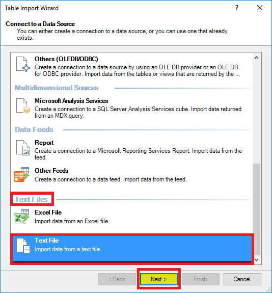

Step 3: And on the next screen, we must need to provide the path on which the text file containing data is physically located, and then we will mention how to save the data file to import under the File Path option. After that, we will click the Browse… button and then navigate through the path respectively.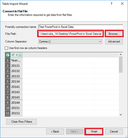

We must ensure that we have selected that Tab as a "Column Separator," then we will check the option for Use the first row as column headers options.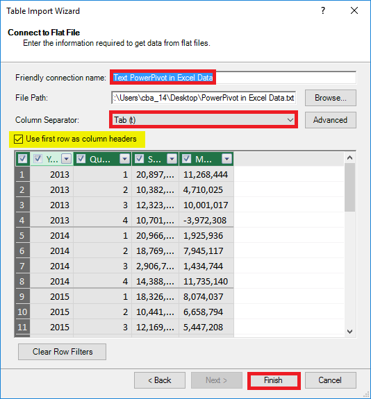

As per the above step, the first will allow the data to be get spread across different columns, while the second will consider the first row from our selected data as a column header. Just after that, we will click on the Finish button, and by doing this, we will see that the respective selected amount of the data is loaded under PowerPivot, as depicted below.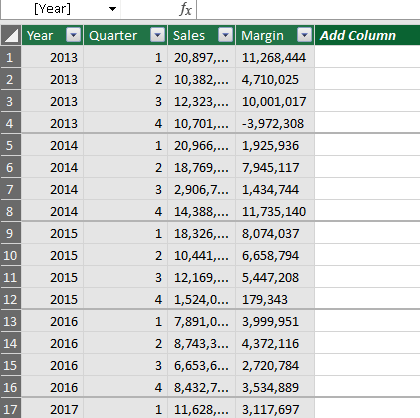

How we can add a Calculated Column under PowerPivot Data?

Calculated column can also be added under the PowerPivot. As in our example, we have Sales and Margin values, and by considering these two columns, we can easily compute the achieved margin and can store it in the new column under the PowerPivot.

To achieve this we are required to follow down the below-mentioned steps:

Step 1: In the very first step, under the PowerPivot, we can see a blank "Add Column" just after all of our data columns, and this column will allow us to add some computed data to it.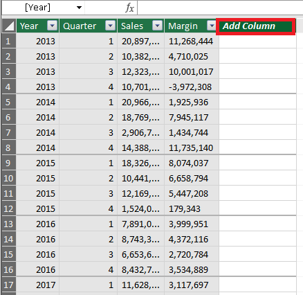

Step 2: After that, we must rename this blank column as Margin% by double-clicking on the "Add Column" row.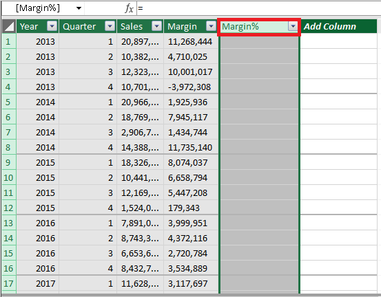

Step 3: Now in the very first cell of column Margin%, we can make use of the formula as Margin or Sales using "Equals to sign." The formula structure in PowerPivot is different as it is nothing but a pivot table.

Formula: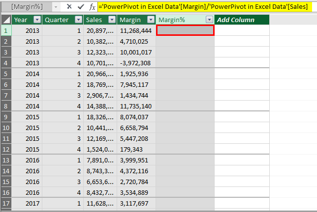

='PowerPivot in Excel Data'[Margin]/'PowerPivot in Excel Data'[Sales]

Step 4: Now we are required to press the Enter key; just after pressing the Enter Key from the keyboard, we can see that all the active rows will be get added with the same formula, and the Margin% will be calculated.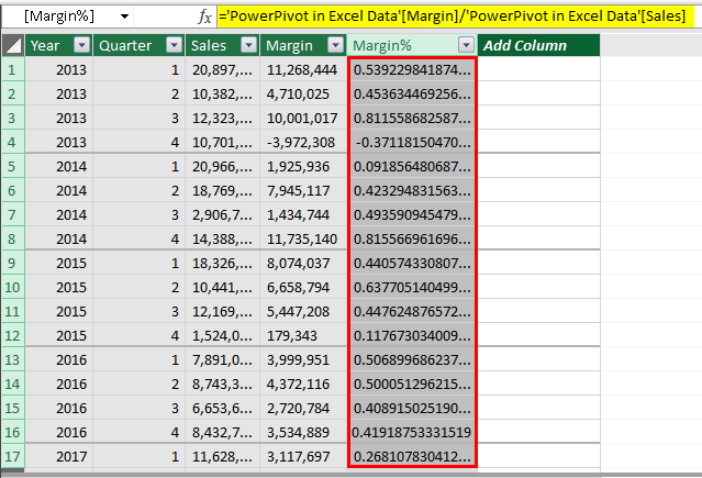

Step 5: After performing the above steps, we are required to format the Margin% column as % by using the formatting tab in PowerPivot.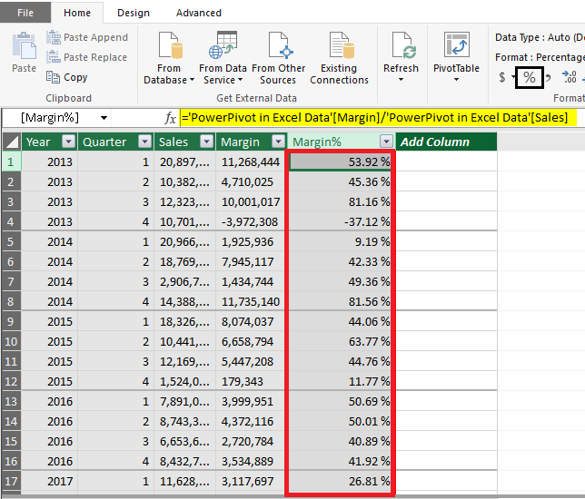

And by performing all the above step we can easily add calculated columns under the PowerPivot.

What things need to be remembered about PowerPivot in Microsoft Excel?

The important things which need to be remembered by an individual while working with the PowerPivot are as follows:

1. It is quite mandatory to clean the data before an individual imports it under the PowerPivot. And then the individual can easily make use of the other Excel formulae, which can be effectively used for the purpose of cleaning the Microsoft Excel data.
   • Example: Right, Left, Trim, it also, removes duplicates and can convert numbers and dates into a proper format.
2. And if in case an individual imports two or more tables in PowerPivot, then in that case it will be automatically creating the Data Model.
3. An individual can also add calculated column fields in the PowerPivot as done in Excel.